Download
1 / 85
1.1k likes | 1.89k Views
Chapter 3 Graphics Output Primitives Some slides adapted from Benjamin Lok, Ilmi Yoon and Falko Kuester. Glossary. CG API – Computer Graphics Application Programming Interface tbs – to be specified FoV – Field of View +’s – pluses, advanatges

E N D
Chapter 3 Graphics Output Primitives Some slides adapted from Benjamin Lok, Ilmi Yoon and Falko Kuester Expanded by Jozef Goetz
Glossary • CG API – Computer Graphics Application Programming Interface • tbs – to be specified • FoV – Field of View • +’s – pluses, advanatges • -’s – minuses, disadvantages • Orthogonal to = Normal to = forms a 90o angle with • Norm of a vector = length of the vector • Are coplanar = there is a plane containing them Expanded by Jozef Goetz
Glossary • Aliasing is the jagged edges on curves and diagonal lines in a bitmap image. • Anti-aliasing is the process of smoothing out those jaggies. • Graphics software programs have options for anti-aliasing text and graphics. • Enlarging a bitmap image accentuates the effect of aliasing. Expanded by Jozef Goetz
Outline • 3-1Coordinate Reference Frames , • 3-2Specifying a Two-Dimensional -World-Coordinate Reference Frame in OpenGL • 3-3OpenGL Point Functions • 3-4OpenGL Line Functions • 3-5Line-Drawing Algorithms • 3-6Parallel Line Algorithms • 3-7Setting Frame-Buffer Values • 3-8OpenGL Curve Functions • 3-9Circle-Generating Algorithms • 3-10Ellipse-Generating Algorithms • 3-11Other Curves • 3-12Parallel Curve Algorithms • 3-13Pixel Addressing and ObjectGeometry Expanded by Jozef Goetz
Outline • 3-14Fill-Area Primitives • 3-15Polygon Fill Areas • 3-16OpenGL Polygon Fill-AreaFunctions • 3-17OpenGL Vertex Arrays • 3-18Pixel-Array Primitives • 3-19OpenGL Pixel-Array Functions • 3-20Character Primitives • 3-21OpenGL Character Functions • 3-22Picture Partitioning • 3-23OpenGL Display Lists • 3-24OpenGL Display-Window ReshapeFunction • 3-25Summary Expanded by Jozef Goetz
Basic Elements • Geometry is the study of the relationships among objects in an n-dimensional space • In computer graphics, we are interested in objects that exist in 3 dimensions • Want a minimum set of primitives from which we can build more sophisticated objects • Geometry provides a mathematical foundation for much of computer graphics. Expanded by Jozef Goetz
Coordinate-Free Geometry • When we learned simple geometry, most of us started with a Cartesian approach • Points were at locations in space p=(x,y,z) • We derived results by algebraic manipulations involving these coordinates • Physically, points exist regardless of the location of an arbitrary coordinate system • Most geometric results are independent of the coordinate system • Euclidean geometry: two triangles are identical if two corresponding sides and the angle between them are equal Expanded by Jozef Goetz
Basic Elements We will need: • Three basic elements • Scalars • Vectors • Points • Develop mathematical operations among them • Define basic primitives: • Line segments • Polygons Expanded by Jozef Goetz
Basic Elements • Points are associated with locations of • Vectors represent displacements between points or directions • Points, vectors, and operators that combine them are the common tools for solving many geometric problems that arise in • Geometric Modeling, • Computer Graphics, • Animation, • Visualization, and • Computational Geometry. Expanded by Jozef Goetz
3.1 COORDINATE REFERENCE FRAMES To describe a picture, we first decide upon • A convenient Cartesian coordinate system, called the world-coordinate reference frame, which could be either 2D or 3D. • We then describe the objects in our picture by giving their geometricspecifications in terms of positions in world coordinates. • e.g., we define a straight-line segment with two endpoint positions, and a polygon is specified with a set of positions for its vertices. • These coordinate positions are stored in the scene descriptionalong with other info about the objects, such as their color and their coordinateextents, • which are the minimum and maximumx, y, and z values for each object. • A set of coordinateextents is also described as a boundingboxfor an object. • For a 2D figure, the coordinate extents are sometimes called an object's bounding rectangle. Expanded by Jozef Goetz
3.1 COORDINATE REFERENCE FRAMES • Objects are then displayed by passing the scenedescriptionto the viewing routines, • which identify visible surfaces • and map the objectsto the frame bufferpositions and then on the video monitor. • The scan-conversion algorithmstoresinfoabout the scene, such as color values, at the appropriate locationsin the frame buffer, and the objects in the scene are displayed on the output device. • locations on a video monitor • are referenced in integer screen coordinates, which • correspond to the integer pixel positions in the frame buffer. Expanded by Jozef Goetz
3.1 COORDINATE REFERENCE FRAMES • E.g. scan-line algorithms for the graphics primitives use the coordinate descriptions to determine the locations of pixels • e.g. given the endpoint coordinates for a line segment, a display algorithm must calculate the positions for those pixels that liealong the line pathbetween the endpoints. • Since a pixel position occupies a finite area of the screen, • the finite size of a pixel must be taken into account by the implementation algorithms. • for the present, we assume that each integer screen position references the center of a pixel area. Expanded by Jozef Goetz
3.1 COORDINATE REFERENCE FRAMES • Once pixel positions have been identified the color values must be stored in the frame buffer • Assume we have available a low-level procedure of the form setPixel (x, y); stores the current color setting into the frame buffer at integer position (x, y), relative to the selected position of the screen-coordinate origin getPixel (x, y, color); retrieve the currentframe-buffer setting for a pixel location; • parameter color receives an integer value corresponding to the combined RGB bit codes stored for the specified pixel at position (x, y). • additional screen-coordinate information is needed for 3D scenes. For a two-dimensional scene, all depth values are 0. Expanded by Jozef Goetz
3.1 Absolute and Relative Coordinate Specifications • we have discussed are stated as absolutecoordinate values • some graphics packages also allow positions to be specified using relativecoordinates • as an offset from the last position that was referenced (called the current position) Expanded by Jozef Goetz
3-2 SPECIFYING A 2D WORLD-COORDINATE REFERENCE FRAME IN OpenGL • World-coordinate limits for a display window, as specified in the glOrtho2D function. • gluOrtho2D function specifies an orthogonal projection, we need also to be sure that the coordinate values are placed in the OpenGL projection matrix. • In addition, we could assign the identity matrix as the projection matrix before defining the world-coordinate range. • This would ensure that the coordinate values were not accumulated with any values we may have previouslyset for the projection matrix. glMatrixMode (GL_PROJECTION); glLoadIdentity ( ); glu0rtho2D (xmin, xmax, ymin, ymax); • The display window will then be referenced by coordinates (xmin, ymin)at the lower-left corner and by coordinates (xmax, ymax)at the upper-right corner, as shown in Fig. 3-2. Expanded by Jozef Goetz
3-3 QpenGL POINT FUNCTIONS • To specify the geometry of a point, we simply give a coordinate positionin the world reference frame. • Then along with other geometric descriptions is passed to the viewing routines. • Unless we specify other attribute values, OpenGL primitives are displayed with a default size and color. • The defaultcolor for primitives is white and the defaultpointsize is equal to the size of one screen pixel. Expanded by Jozef Goetz
3-3 QpenGL POINT FUNCTIONS • A glVertex function must be placed between a glBegin function and a glEnd function. • The argument of the glBegin function is used to identify the kind of output primitive that is to be displayed, • For point plotting, the argument of the g1Begin function is the symbolic constant GL_POINTS. • and glEnd takes no arguments. glBegin (GL_POINTS); glVertex* ( ); glEnd ( ) ; Expanded by Jozef Goetz
3-3 QpenGL POINT FUNCTIONS glVertex* ( ); • state the coordinate values for a single position • where the asterisk (*) indicates that suffix codes are required for this function. • These suffix codes are used to identify the spatial dimension, 2, 3, or 4 (indicates a scaling factor for the Cartesian-coordinate values.) • any (x, y) coordinate specification is equivalent to (x, y, 0) with h = 1 • the numerical data type • i (integer), s (short), f (float), and d (double) • and a possible vector form for the coordinate specification • append a third suffix code: v (for "vector"). • the glVertex function is used in OpenGL to specify coordinates for anypoint position. • In this way, a single function is used for point, line, and polygon specifications Expanded by Jozef Goetz
3-3 QpenGL POINT FUNCTIONS. glBegin (GL_POINTS); glVertex2i (50, 100); glVertex2i (75, 150); glVertex2i (100, 200); g1End ( ) ; • Alternatively, we could specify the coordinate values for the preceding points in arrays such as int pointl [ ] = {50, 100); int point2 [ ] = {75, 150); int point3 [ ] = {100, 200}; and call the OpenGL functions for plotting the three points as glBegin (GL_POINTS); glVertex2iv (pointl); glVertex2iv (point2); glVertex2iv (point3); glEnd ( ) ; Expanded by Jozef Goetz
3-3 QpenGL POINT FUNCTIONS • And here is an example of specifying two point positions in a 3D world reference frame. In this case, we give the coordinates as explicit floating-point values. glBegin (GL-POINTS); glVertex3f (-78.05, 909.72, 14.60); glVertex3f (261.91, -5200.67, 188.33); glEnd ( ) ; Expanded by Jozef Goetz
3-3 QpenGL POINT FUNCTIONS. class wcPt2D { public: GLfloat x, y; }; • Using this class definition, we could specify a 2D, world-coordinate point position with the statements wcPt2D pointPos; pointPos.x = 120.75; pointPos.y = 45.30; glBegin (GL_POINTS); glVertex2f (pointPos.x, pointPos.y); glEnd ( ) Expanded by Jozef Goetz
3-4 OpenGL LINE FUNCTIONS • now we use a symbolic constant as the argument for the g1Begin function that interprets a list of positionsas the endpoint coordinates for line segments. • A set of straight-line segments between each successive pair of endpoints in a list is generatedusing the primitive line constant GL_LINES glBegin (GL_LINES): glVertex2iv(pl); glVertex2iv(p2); glVertex2iv(p3); glVertex2iv(p4); glVertex2iv(p5); glEnd ( ); • Nothing is displayed if we do not list at least two coordinate positions p3 pl p2 p4 Expanded by Jozef Goetz
3-4 OpenGL LINE FUNCTIONS. glBegin (GL_LINE_STRIP); glVertex2iv (pl);glVertex2iv (p2);glVertex2iv (p3);glVertex2iv (p4);glVertex2iv (p5): glEnd ( ) • The first line segment in the polyline is displayed between the first endpoint and the second endpoint; • the second line segment is between the second and third endpoints; and so forth, up to the last line endpoint. Expanded by Jozef Goetz
3-4 OpenGL LINE FUNCTIONS giBegin (GL_LINE_LOOP);glVertex2iv (pl);glVertex2iv (p2);glVertex2iv (p3);glVertex2iv (p4);glVertex2iv (p5); glEnd ( ) ; • produces a closed polyline. • the lastcoordinate endpoint in the sequence is connected to the first coordinate endpoint of the polyline. Expanded by Jozef Goetz
3-5 LINE-DRAWING ALGORITHM A straight-line segmentin a scene is defined by the coordinate positions for the endpoints of the segment. • To display the line on a raster monitor, the graphics system must • first project the endpoints to integer screen coordinates and • determine the nearest pixel positions along the line path between the two endpoints. • Then the line color is loaded into the frame buffer at the corresponding pixel coordinates. • Reading from the frame buffer, the video controller plots the screen pixels. • This process digitizes the line into a set of discrete integer positions that, in general, only approximates the actual line path. Expanded by Jozef Goetz
3-5 LINE-DRAWING ALGORITHM • On raster systems, lines are plotted with pixels, and step sizesin the horizontal and vertical directions are constrained by pixel separations. • That is, we must "sample" a line at discrete positions and determine the nearest pixelto the line at sampled position. • Sampling is measuring the values of the function at equal intervals • Idea: A line is sampled at unit intervals in one coordinate and the corresponding integer values nearest the line path are determined for the other coordinate. Expanded by Jozef Goetz
Towards the Ideal Line • We can only do a discrete approximation • Illuminate pixels as close to the true path as possible, consider bi-level display only • Pixels are either lit or not lit Expanded by Jozef Goetz
<Main Concept> • In the raster line alg., • we sample at unit intervals and • determine theclosest pixel position to the specified line path at each step Expanded by Jozef Goetz
What is an ideal line • Must appear straight and continuous • Only possible axis-aligned and 45o lines • Must interpolate bothdefining end points • Must have uniform density and intensity • Consistent within a line and over all lines • What about anti-aliasing? • Aliasing is the jagged edges on curves and diagonal lines in a bitmap image. • Anti-aliasing is the process of smoothing out those jaggies. • Graphics software programs have options for anti-aliasing text and graphics. • Enlarging a bitmap image accentuates the effect of aliasing. • Must be efficient, drawn quickly • Lots of them are required!!! Expanded by Jozef Goetz
Simple Line • The Cartesian slope-intercept equation for a straight line is: • y = mx + b • with mas the slope of the line and bas the yintercept. • Simple approach: • increment x, solve for y • -‘s: Floating point arithmetic required Expanded by Jozef Goetz
Does it Work? • It seems to work okay for lines with a slope m <= 1 • but doesn’t work well for lines with slope m >= 1 • lines become more discontinuous in appearance if we sample at unit x intervals • and we must add more than 1 pixel per column to make it work. • Solution? - 1. use symmetry. Expanded by Jozef Goetz
Modify algorithm per octant OR 2. use: increment along x-axis if dy<dx (e.g. m<1) else increment along y-axis We will use approach 2 Expanded by Jozef Goetz
Digital Differential Analyzer DDA alg. #include <stdlib.h> #include <math.h> inline int round (const float a) { return int (a + 0.5); } void lineDDA (int x0, int y0, int xEnd, int yEnd) { int dx = xEnd - x0, dy = yEnd - y0, steps, k; float xIncrement, yIncrement, x = x0, y = y0; // find max {dx, dy} if (fabs (dx) > fabs (dy)) // for m <=1 // for m >1 steps = fabs (dx); // # of x units // = steps // ------- = skipped else steps = fabs (dy); // # of y units // ------- // = steps xIncrement = float (dx) / float (steps); // dx = 1 // dx = 1/m or -1/m yIncrement = float (dy) / float (steps); // dy = m or –m // dy = 1 setPixel (round (x), round (y)); //stores the current color setting into the frame buffer // at integer position (x, y), for (k = 0; k < steps; k++) { x += xIncrement; // x += 1; // x = x + 1/m or -1/m y += yIncrement; // y = y + m or -m // y += 1; setPixel (round (x), round (y)); } } Expanded by Jozef Goetz
-’s of DDA algorithm • Still need a lot of floating point arithmetic which is stilltime consuming. • 2 ‘round’s and 2 adds per pixel. • Is there a simpler way ? • Can we use only integer arithmetic ? • Easier to implement in hardware. Expanded by Jozef Goetz
Bresenham’s line Algorithm • we introduce an accurate and efficientraster line-generating algorithm, • that uses only incremental integer calculations. • in addition, Bresenham's line algorithm can be adapted to display circles and other curves. Expanded by Jozef Goetz
Observation on lines. while( n-- ) { draw(x,y); move right; if( below line ) move up; } • Another approach will be applied: • decide which of two possible pixel positions is • closer to the of a display screen at each sample step. • e.g. starting from the left endpoint Expanded by Jozef Goetz
To illustrate Bresenham's approach, we first consider the scan-conversion process for lines with positive m < 1.0. • Pixel positions along a line path are then determined by sampling at unit x intervals. • Starting from the left endpoint (xo, yo) of a given line, we step to each successive column (x position) and plot the pixel whose scan-line y value is closest to the line path. • Figure 3-10 demonstrates the kth step in this process. • Assuming we have determined that the pixel at (x[k], y[k]) is to be displayed, • we next need to decide which pixel to plot in column x[k+1]? • Our choices are the pixels at positions (x[k+1], y[k])and • (x[k+1], y[k+1]). Expanded by Jozef Goetz
Idea: test the sign of an integer parameter whose value is proportional to the difference between the vertical separations of the two pixel positions from the actual line path. Expanded by Jozef Goetz
Bresenham’s Line Algorithm • An implementation for slopes in the range 0 < m < 1.0 is given here. • Endpoint pixel positions for the line are passed to this procedure, and pixels are plotted from the leftendpoint to the rightendpoint. #include <stdlib.h> #include <math.h> /* Bresenham line-drawing procedure for |m| < 1.0. */ void lineBres (int x0, int y0, int xEnd, int yEnd) { int dx = fabs (xEnd - x0), dy = fabs(yEnd - y0); int p = 2 * dy - dx; // calculate initial value of a decision parameter int twoDy = 2 * dy, twoDyMinusDx = 2 * (dy - dx); int x, y; /* Determine which endpoint to use as start position. */ if (x0 > xEnd) { x = xEnd; y = yEnd; xEnd = x0; } else { x = x0; y = y0; } setPixel (x, y); // draw the first point while (x < xEnd) { x++; if (p < 0) p += twoDy; // no y change else { y++; p += twoDyMinusDx; } setPixel (x, y); } } Expanded by Jozef Goetz
Bresenham’s Line Algorithm To illustrate the algorithm, we digitize the line with endpoints (20, 10)and (30, 18) This line has a slope of 0.8, with dx =10,dy =8 The initial decision parameter has the value: p = 20dy – dx = 6 and the increments for calculating successive decision parameters are 20dy = 16, 2dy – 2dx = -4 • We plot the initial point = (20, 10), and determine successive pixel positions along the line path from the decision parameter as: k 0 6 (21, 11) 1 2 (22, 12) 2 -2 (23, 12) 3 14 (24, 13) 4 10 (25, 14) 5 6 (26, 15) 6 2 (27, 16) 7 -2 (28, 16) 8 14 (29, 17) 9 10 (30, 18) • Pixel positions along the line path between endpoints • (20, 10) and (30, 18), plotted with Bresenham's line algorithm. Expanded by Jozef Goetz
Bresenham’s Line Algorithm • Bresenham's algorithm is generalized to lines with arbitrary slope by considering the symmetry between the variousoctants and quadrants of the xyplane. • For a line with positivem > 1.0, we interchange the roles of the x and y directions. • i.e. we step along the ydirection in unit steps and calculatesuccessivexvaluesnearest the line path. • Also, we could revise the program to plotpixels starting from either endpoint. • If the initial position for a line with positiveslope is the rightendpoint, both xand ydecrease as we stepfrom right to left • For negative slopes, the procedures are similar, except that now one coordinate decreases as the other increases. Expanded by Jozef Goetz
Displaying Polylines • Implementation of a polyline procedure is accomplished by invoking a linedrawing routine n - 1 times to display the lines connecting the n endpoints. • Each successive call passes the coordinate pair needed to plot the next line section, where the firstendpoint of each coordinate pair is the lastendpoint of the previous section. Expanded by Jozef Goetz
3-6 PARALLEL LINE ALGORITHMS • The line-generating algorithms so far determine pixel positions sequentially. • Using parallel processing, we can calculate multiple pixel positions along a line path simultaneously by partitioning the computations among the variousprocessors available. • An important consideration in devising a parallelalgorithm is to balance the processing load among the available processors. Expanded by Jozef Goetz
3-6 PARALLEL LINE ALGORITHMS • I. Given processors, we can set up a parallel Bresenham line algorithm by subdividing the line path into partitions and simultaneously generating line segments in each of the subintervals. • For a line with slope 0 < m < 1.0 and left endpoint coordinate position (x0, y0) , we partition the line along the positivexdirection. Expanded by Jozef Goetz
3-6 PARALLEL LINE ALGORITHMS • The distance between beginning x positions of adjacent partitions i.e. partition width where = width of the line = # of processors • Numbering the partitions, and the processors, as 0, 1, 2, up to - 1, we calculate the starting x coordinate for the k-th partition as Expanded by Jozef Goetz
3-6 PARALLEL LINE ALGORITHMS • The change in the y direction over each partition is calculated from the line slope m and partition width : • At the k-th partition, the starting y coordinate is then • the initial value for the decision parameter was • so for each partition we get Expanded by Jozef Goetz
3-6 PARALLEL LINE ALGORITHMS • Each processor then calculatespixelpositions over its assignedsubinterval using the preceding startingdecision parameter value and the startingcoordinates . • Floating-point calculations can be reduced to integer arithmetic in the computations for startingvalues and by substituting and rearranging terms. • We can extend the parallel Bresenham algorithm for m > 1.0 by partitioning the line in the y direction and calculating beginning xvaluesfor the partitions. • For negative slopes, we increment coordinate values in one direction and decrement in the other. Expanded by Jozef Goetz
3-6 Another PARALLEL LINE ALGORITHMS • II. Assign each processor to a particular group of screen pixels. • each assigned processor to one pixel within some screen region (within the limits of the coordinate extents of the line) calculates pixel distances from the line path. • III. Assign to each processor either a scan line or a column of pixelsdepending on the line slope. • Each processor then calculates the intersection of the line with the horizontal row or vertical column of pixels assigned to that processor. • For a line with slope abs (m) < 1.0, each processor simply solves the line equation for y, given an x column value. • For a line with slope magnitude m > 1.0, the lineequation is solved for x by each processor, given a scan line y value. • Such direct methods, although slow on sequential machines, can be performed efficiently using multiple processors. Expanded by Jozef Goetz