OutPut Primitives

1. OutPut Primitives By : Engr. Syed Atir Iftikhar Compile by : Engr. Syed Atir Iftikhar

2. Basic Graphics System Output device Input devices Image formed in FB [Edward Angel, Interactive computer Graphics, 2009] Compile by : Engr. Syed Atir Iftikhar

3. Raster Graphics Compile by : Engr. Syed Atir Iftikhar

4. Frame Buffer Compile by : Engr. Syed Atir Iftikhar

5. Frame Buffer Refresh • Refresh Rate • Usually 30~75 Hz Compile by : Engr. Syed Atir Iftikhar cgvr.korea.ac.kr

6. Color CRT Compile by : Engr. Syed Atir Iftikhar cgvr.korea.ac.kr

7. LINE-DRAWING ALGORITHMS Compile by : Engr. Syed Atir Iftikhar

8. LINE-DRAWING ALGORITHMS Compile by : Engr. Syed Atir Iftikhar

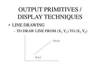
9. LINE-DRAWING ALGORITHMS • LINE-DRAWING ALGORITHMS • The Cartesian slope-intercept equation for a straight line is • y = m . x + b • with m representing the slope of the line and b as they intercept. Given that the two endpoints of a line segment are specified at positions (x1, y1,) and (x2 , y2), as shown in Fig. we can determine values for the slope m and y intercept b with the following calculations: Y2 Y1 Fig 3.3 x1x2 Compile by : Engr. Syed Atir Iftikhar

10. LINE-DRAWING ALGORITHMS • m = y2 – y1 eq 3.2 x2 – x1 • b = y1 – m . X1 eq 3.3 • Algorithms for displaying straight lines are based on the line equation(the dotted values) and the calculations is done by above formulas. • For any given x interval x along a line, we can compute the corresponding y interval y from Eq 3.2 as • y = m x Compile by : Engr. Syed Atir Iftikhar

11. LINE-DRAWING ALGORITHMS • Similarly, we can obtain the x interval x corresponding to a specified y as • x = y m • These equations form the basis for determining deflection voltages in analog devices. Compile by : Engr. Syed Atir Iftikhar

12. LINE-DRAWING ALGORITHMS • Numerical example of finding slope m: • (Ax, Ay) = (23, 41), (Bx, By) = (125, 96) Compile by : Engr. Syed Atir Iftikhar

13. Output Primitives • Points • Lines • DDA Algorithm • Bresenham’s Algorithm • Polygons • Scan-Line Polygon Fill • Inside-Outside Tests • Boundary-Fill Algorithm • Antialiasing Compile by : Engr. Syed Atir Iftikhar

14. Points • Single Coordinate Position • Set the bit value(color code) corresponding to a specified screen position within the frame buffer y setPixel (x, y) x Compile by : Engr. Syed Atir Iftikhar

15. Lines • Intermediate Positions between Two Endpoints • DDA, Bresenham’s line algorithms Compile by : Engr. Syed Atir Iftikhar

16. DDA Algorithm • The digital differential analyzer (DDA) is a scan-conversion line algorithm based on calculating either y or x, • Case 1: • Consider first a line with positive slope, as shown in Fig. 3-3. If the slope is less than or equal to 1, we sample at unit x intervals ( x = 1) and compute each successive y value as Compile by : Engr. Syed Atir Iftikhar

17. y2 y1 x1 x2 DDA Algorithm • Digital Differential Analyzer • 0 < Slope <= 1 • Unit x interval = 1 • Subscript k takes integer values starting from 1, for the first point, and increases by 1 until the final endpoint is reached. Since m can be any real number between 0 and 1, the calculated y values must be rounded to the nearest integer. Equation 3.6 Compile by : Engr. Syed Atir Iftikhar

18. y2 y1 x1 x2 DDA Algorithm • Digital Differential Analyzer • 0 < Slope <= 1 • Unit x interval = 1 • Slope > 1 • Unit y interval = 1 • For lines with a positive slope greater than 1 we reverse the roles of x and y. That is, we sample at unit y intervals ( y = 1) and calculate each succeeding x value as Equation 3.7 Compile by : Engr. Syed Atir Iftikhar

19. y1 y2 x1 x2 DDA Algorithm • Digital Differential Analyzer • 0 < Slope <= 1 • Unit x interval = 1 • Slope > 1 • Unit y interval = 1 • -1 <= Slope < 0 • Unit x interval = -1 • Equations 3-6 and 3-7 are based on the assumption that lines are to be processed from the left endpointto the right endpoint (Fig. 3-3). If this processing is reversed,so that the starting endpoint is at the right, then either we have x = -1 Equation 3.8 Compile by : Engr. Syed Atir Iftikhar

20. y2 y1 x1 x2 DDA Algorithm • Digital Differential Analyzer • Slope >= 1 • Unit x interval = 1 • 0 < Slope < 1 • Unit y interval = 1 • -1 <= Slope < 0 • Unit x interval = -1 • Slope < -1 • Unit y interval = -1 or (when the slope is greater than 1) Equation 3.9 we have y = -1 with Compile by : Engr. Syed Atir Iftikhar

21. DDA Algorithm • Advantages • DDA algorithm is a faster method for calculating the pixel positions than the direct use of line equation. • It eliminates multiplication by making use of raster characteristics. Compile by : Engr. Syed Atir Iftikhar

22. DDA Algorithm • Disadvantages • DDA algorithm runs slowly because it requires real arithmetic (floating point operations) and rounding operations Compile by : Engr. Syed Atir Iftikhar

23. DDA versus Bresenham’s Algorithm The Bresenham line algorithm has the following advantages: • An fast incremental algorithm • Uses only integer calculations Comparing this to the DDA algorithm, DDA has the following problems: • Accumulation of round-off errors can make the pixelated line drift away from what was intended • The rounding operations and floating point arithmetic involved are time consuming Compile by : Engr. Syed Atir Iftikhar

24. Bresenham’s Line Algorithm • Midpoint Line Algorithm • Decision variable • d > 0 : choose NE • : dnew= dold+a+b • d <= 0 : choose E • : dnew= dold+a NE Q M P(xp, yp) E Compile by : Engr. Syed Atir Iftikhar

25. Bresenham’s Algorithm(cont.) • Initial Value of d • Update d Compile by : Engr. Syed Atir Iftikhar

26. Bresenham’s Algorithm(cont.) • BRESENHAM’S LINE DRAWING ALGORITHM(for |m| < 1.0) • Input the two line end-points, storing the left end-point in (x0, y0) • Plot the point (x0, y0) • Calculate the constants Δx, Δy, 2Δy, and (2Δy - 2Δx) and get the first value for the decision parameter as: • At each xk along the line, starting at k = 0, perform the following test. If pk < 0, the next point to plot is (xk+1, yk) and: Compile by : Engr. Syed Atir Iftikhar

27. Bresenham’s Algorithm(cont.) • Otherwise, the next point to plot is (xk+1, yk+1) and: • Repeat step 4 (Δx) times The algorithm and derivation above assumes slopes are less than 1. for other slopes we need to adjust the algorithm slightly. Compile by : Engr. Syed Atir Iftikhar

28. Adjustment For m>1, we will find whether we will increment x while incrementing y each time. After solving, the equation for decision parameter pk will be very similar, just the x and y in the equation will get interchanged. Compile by : Engr. Syed Atir Iftikhar

29. Bresenham’s Algorithm(cont.) • EXAMPLE : • To illustrate the algorithm, we digitize the line with endpoints (20, 10) and (30,18). This line has a slope of 0.8, with • x = 10 , y = 8 Compile by : Engr. Syed Atir Iftikhar

30. (30,18) (20,10) kpk (xk+1,yk+1) 0 6 (21,11) 1 2 (22,12) 2 -2 (23,12) 3 14 (24,13) 4 10 (25,14) 5 6 (26,15) 6 2 (27,16) 7 -2 (28,16) 8 14 (29,17) 9 10 (30,18) Example – Draw a line from (20,10) to (30,18) x = 10 y = 8 initial decision parameter has the value p0 = 2 y – x = 6 Increment for calculating successive decision parameter are 2 y = 16, 2 y – 2 x) = -4 Compile by : Engr. Syed Atir Iftikhar

31. Bresenham’s Algorithm(cont.) 20 , 10 If pk < 0, the next point to plot is (xk+1, yk) and: Compile by : Engr. Syed Atir Iftikhar

32. Bresenham’s Algorithm(cont.) • Go through the steps of the Bresenham line drawing algorithm for a line going from (21,12) to (29,16) Compile by : Engr. Syed Atir Iftikhar

33. Circle : • Drawing a circle on the screen is a little complex than drawing a line. There are two popular algorithms for generating a circle − Bresenham’s Algorithm and Midpoint Circle Algorithm. These algorithms are based on the idea of determining the subsequent points required to draw the circle. Let us discuss the algorithms in detail − • In computer graphics, the midpoint circle algorithm is an algorithm used to determine the points needed for rasterizing a circle. Bresenham's circle algorithm is derived from the midpoint circle algorithm. Compile by : Engr. Syed Atir Iftikhar

34. A Simple Circle Drawing Algorithm The equation for a circle is: where r is the radius of the circle So, we can write a simple circle drawing algorithm by solving the equation for y at unit x intervals using: Compile by : Engr. Syed Atir Iftikhar

35. A Simple Circle Drawing Algorithm (cont…) Compile by : Engr. Syed Atir Iftikhar

36. A Simple Circle Drawing Algorithm (cont…) However, unsurprisingly this is not a brilliant solution! Firstly, the resulting circle has large gaps where the slope approaches the vertical Secondly, the calculations are not very efficient • The square (multiply) operations • The square root operation – try really hard to avoid these! We need a more efficient, more accurate solution Compile by : Engr. Syed Atir Iftikhar

37. Polar coordinates X=r*cosθ+xc Y=r*sinθ+yc 0º≤θ≤360º Or 0 ≤ θ ≤6.28(2*π) Problem: • Deciding the increment in θ • Cos, sin calculations Compile by : Engr. Syed Atir Iftikhar

38. (-x, y) (x, y) (-y, x) (y, x) (-y, -x) (y, -x) (-x, -y) (x, -y) Eight-Way Symmetry The first thing we can notice to make our circle drawing algorithm more efficient is that circles centred at (0, 0) have eight-way symmetry Compile by : Engr. Syed Atir Iftikhar

39. Mid-Point Circle Algorithm Similarly to the case with lines, there is an incremental algorithm for drawing circles – the mid-point circle algorithm In the mid-point circle algorithm we use eight-way symmetry so only ever calculate the points for the top right eighth of a circle, and then use symmetry to get the rest of the points The mid-point circle algorithm was developed by Jack Bresenham, who we heard about earlier. Bresenham’s patent for the algorithm can be vied Compile by : Engr. Syed Atir Iftikhar

40. 6 5 4 3 1 2 3 4 Mid-Point Circle Algorithm (cont…) Compile by : Engr. Syed Atir Iftikhar

41. 6 M 5 4 3 1 2 3 4 Mid-Point Circle Algorithm (cont…) Compile by : Engr. Syed Atir Iftikhar

42. 6 M 5 4 3 1 2 3 4 Mid-Point Circle Algorithm (cont…)

43. (xk+1, yk) (xk, yk) (xk+1, yk-1) Mid-Point Circle Algorithm (cont…) Assume that we have just plotted point (xk, yk) The next point is a choice between (xk+1, yk) and (xk+1, yk-1) We would like to choose the point that is nearest to the actual circle So how do we make this choice? Compile by : Engr. Syed Atir Iftikhar

44. Mid-Point Circle Algorithm (cont…) Let’s re-jig the equation of the circle slightly to give us: The equation evaluates as follows: By evaluating this function at the midpoint between the candidate pixels we can make our decision Compile by : Engr. Syed Atir Iftikhar

45. Mid-Point Circle Algorithm (cont…) Assuming we have just plotted the pixel at (xk,yk) so we need to choose between (xk+1,yk) and (xk+1,yk-1) Our decision variable can be defined as: If pk < 0 the midpoint is inside the circle and and the pixel at yk is closer to the circle Otherwise the midpoint is outside and yk-1 is closer Compile by : Engr. Syed Atir Iftikhar

46. Mid-Point Circle Algorithm (cont…) To ensure things are as efficient as possible we can do all of our calculations incrementally First consider: or: where yk+1 is either yk or yk-1 depending on the sign of pk Compile by : Engr. Syed Atir Iftikhar

47. Mid-Point Circle Algorithm (cont…) The first decision variable is given as: Then if pk < 0 then the next decision variable is given as: If pk > 0 then the decision variable is: Compile by : Engr. Syed Atir Iftikhar

48. The Mid-Point Circle Algorithm MID-POINT CIRCLE ALGORITHM • Input radius r and circle centre (xc, yc), then set the coordinates for the first point on the circumference of a circle centred on the origin as: • Calculate the initial value of the decision parameter as: • Starting with k = 0 at each position xk, perform the following test. If pk< 0, the next point along the circle centred on (0, 0) is (xk+1, yk) and: Compile by : Engr. Syed Atir Iftikhar

49. The Mid-Point Circle Algorithm (cont…) Otherwise the next point along the circle is (xk+1, yk-1) and: Where 2x k+1 = 2xk + 2 and2yk+1 = 2yk - 2 • Determine symmetry points in the other seven octants • Move each calculated pixel position (x, y) onto the circular path centred at (xc, yc) to plot the coordinate values: • Repeat steps 3 to 5 until x >= y Compile by : Engr. Syed Atir Iftikhar

50. Mid-Point Circle Algorithm Example To see the mid-point circle algorithm in action lets use it to draw a circle centred at (0,0) with radius 10 Compile by : Engr. Syed Atir Iftikhar