Download
1 / 24
240 likes | 350 Views
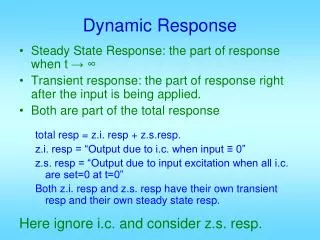
Dynamic Response. Steady State Response: the part of resp. when t →∞ Transient response: the part of resp right after the input is being applied. Both are part of the total resp. total resp = z.i. resp + z.s.resp. z.i. resp = “Output due to i.c. when input ≡ 0”

E N D
Dynamic Response • Steady State Response: the part of resp. when t→∞ • Transient response: the part of resp right after the input is being applied. • Both are part of the total resp. total resp = z.i. resp + z.s.resp. z.i. resp = “Output due to i.c. when input ≡ 0” z.s. resp = “Output due to input excitation when all i.c. are set=0 at t=0”
us(t) 1 0 Typical test signal • Unit step signal: • Unit impulse:δ(t) δ(t) t
Unit ramp: • Unit acc. signal: r(t) t a(t) 0.5 0 1 t
Exponential signal: • sinusoidal: 1 0 t
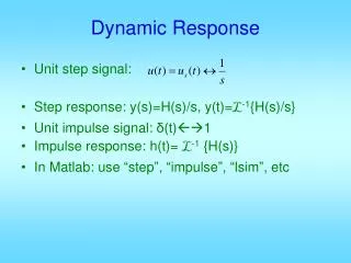
1 s 1 s y(s)=H(s) u(s)= H(s) • Unit step response: In Matlab: step • Unit impulse resp: Matlab: impulse y(s)=H(s) u(s)=1 H(s)
Unit step signal: Step response: y(s)=H(s)/s, y(t)=L-1{H(s)/s} Unit impulse signal: δ(t)1 Impulse response: h(t)= L-1 {H(s)} In Matlab: use “step”, “impulse”, “lsim”, etc Dynamic Response
Defined based on unit step response • Defined for closed-loop system • Steady-state value yss • Steady-state error ess • Settling time ts • = time when y(t) last enters a tolerance band Time domain response specifications
By final value theorem In MATLAB: num = [ .. .. .. .. ] b0 = num(length(num)), or num(end) a0 = den(length(den)), or den(end) yss=b0/a0
If numerical values of y(t) available, abs(y – yss) < tol means inside band abs(y – yss) ≥ tol not inside e.g. t_out = t(abs(y – yss) ≥ tol) contains all those time points when y is not inside the band. Therefore, the last value in t_out will be the settling time. ts=t_out(end)
Peak time tp = time when y(t) reaches its maximum value. Peak value ymax =y(tp) Hence: ymax = max(y); tp = t(y = ymax); Overshoot: OS = ymax - yss Percentage overshoot:
If t50 = t(y >= 0.5·yss), this contains all time points when y(t) is ≥ 50% of yss so the first such point is td. td=t50(1); Similarly, t10 = t(y <= 0.1*yss) & t90 = t(y >= 0.9*yss) can be used to find tr. tr=t90(1)-t10(end)
90%yss 10%yss tr≈0.45 ts ts tp≈0.9sec td≈0.35
±5% ts=0.45 yss=1 ess=0 O.S.=0 Mp=0 tp=∞ td≈0.2 tr≈0.35
tp=0.35 O.S.=0.4 Mp=40% yss=1 es=0 ts≈0.92 td≈0.2 tr≈0.1
Steady-state tracking & sys. types • Unity feedback control: plant + e r(s) y(s) C(s) G(s) - + e r(s) Go.l.(s) y(s) -