Download
1 / 37
370 likes | 519 Views
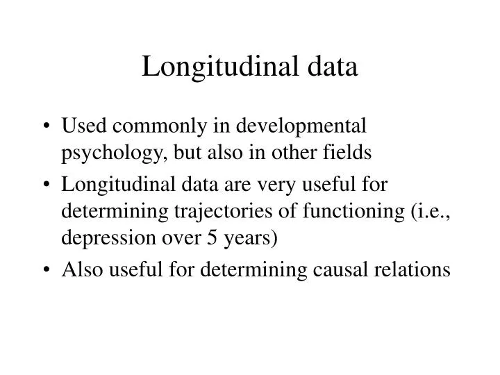
Longitudinal data. Used commonly in developmental psychology, but also in other fields Longitudinal data are very useful for determining trajectories of functioning (i.e., depression over 5 years) Also useful for determining causal relations. My favorite example. Stress. Psycho. adaptation.

E N D
Longitudinal data • Used commonly in developmental psychology, but also in other fields • Longitudinal data are very useful for determining trajectories of functioning (i.e., depression over 5 years) • Also useful for determining causal relations
My favorite example Stress Psycho. adaptation -.58** Note. These data are typically obtained in one point of time, i.e., they are concurrent. Can we draw the arrow as we have here?
Correlation is not causation!(Have we heard that before?) Stress What is the direction of causation, if any exists? Does stress cause poorer psychological adaptation, or the reverse? Can’t tell with these data. Can propose your hypothesis (previous page), but can’t prove this relationship this way. r = -.58** Psycho. adaptation
How about this? Time2 Time1 Stress Psycho. adaptation -.36* R2=.20
Well, there are a lot of variables that might be affecting this relationship Time1 Time2 Stress Psycho. adaptation Psycho. adaptation SES
The recommended method(Pedhazur, 1997): Residualized regression Time1 Time2 Psycho. adaptation Entered first Psycho. adaptation R2=.85 All other variables entered subse- quently SES R2ch=.02 R2ch=.05 Stress Note. However, exogenous variables like SES, gender, etc. may be entered first as covariates.
So, how would it work with the stress and coping paradigm? Time2 Time 1 Stress Stress Psycho. adaptation Psycho. adaptation
How do we assess causality here? Time2 Time 1 Stress Stress Stability & autocorrelation A B Psycho. adaptation Psycho. adaptation Stability & autocorrelation A: Stress1 -> Outcome2 B: Outcome1 -> Stress2
A simpler example: Stability and autocorrelation • Used a dataset by Wheaton et al. (1977), in which they were interested in whether alienation was reasonably stable over a period of 4 years • Latent variable of alienation, made up of anomie and powerlessness • Also curious whether socio-economic status would impact on this stability
Wheaton et al. model e1 e2 e3 e4 Anomie 67 Powerl 67 Anomie 71 Powerl 71 1 l1 1 z1 l2 h1 h2 Alienation 67 b1,1 Alienation 71
Syntax, of course Stability of alienation, First Model: uncorrelated error terms DA NI=6 NO=932 MA=KM KM 11.834 6.947 9.364 6.819 5.091 12.532 4.783 5.028 7.495 9.986 -3.839 -3.889 -3.841 -3.625 9.610 -2.190 -1.883 -2.175 -1.878 3.552 4.503 la anomia67 power67 anomia71 power71 educatin socioind se 1 2 3 4 / MO NY=4 NE=2 BE=SD PS=DI TE=SY le alien67 alien71 FR LY 2 1 LY 4 2 VA 1.0 LY 1 1 LY 3 2 PD OU SE TV MI ND=2
First model: uncorrelated error terms Anomie 67 .31 .69 1.0 Alienation 67 .95 Powerl 67 .37 .77 .33 Anomie 71 1.0 .27 Alienation 71 .91 Powerl 71 R2=.56 .39
How does it fit? • X2(1) = 61.11 • RMSEA = .25 • NFI = .96 • PNFI = .16 • CFI = .96 • RFI = .81 • Crit. N = 102.09 • GFI = .97 • AGFI = .69 • PGFI = .10
What’s da problem? • Would like to allow correlated error . . . • But there’s another problem: namely, there’s only 1 df; can’t allow program to estimate any more parameters. • Ooops, now what? Well, can increase the scope of the model to include other variables, and “borrow” some dfs from those relationships • Two SES variables: education and socioeconomic indicator • Make the model a bit more complex (see next page)
Second model: new latent variable, uncorrelated error terms e1 e2 e3 e4 Anomie 67 Powerl 67 Anomie 71 Powerl 71 1 l1 1 z1 l2 z2 h1 h2 Alienation 67 b1,1 Alienation 71 g2 g1 d1 Education x1 SES 67 1 l3 Socio-econ indicator d2
Second model: uncorrelated error terms Anomie 67 .34 .45 R2=.32 1.0 .31 Alienation 67 1.0 Education 67 -.55* Powerl 67 1.0 .34 SES .68** .30 SEI 67 .78 Anomie 71 -.15* 1.0 .30 Alienation 71 .95 .58 Powerl 71 R2=.58 .36
A better fit? • X2(6) = 71.47 • RMSEA = .11 • NFI = .97 • PNFI = .39 • CFI = .97 • RFI = .92 • Crit. N = 219.99 • GFI = .98 • AGFI = .91 • PGFI = .28 Now, what about correlated error? Would that help?
Third model: 3 latents & correlated error for anomie e1 e2 e3 e4 Anomie 67 Powerl 67 Anomie 71 Powerl 71 1 l1 1 z1 l2 z2 h1 h2 Alienation 67 b1,1 Alienation 71 g2 g1 d1 Education x1 SES 67 1 l3 Socio-econ indicator d2
Now, do we have a better fit? • X2(5) = 6.33 • RMSEA = .02 • NFI = 1.00 • PNFI = .33 • CFI = 1.00 • RFI = .99 • Crit. N = 2218.49 • GFI = 1.00 • AGFI = .99 • PGFI = .24
What about correlated error for powerlessness? • I ran a fourth model, and the change in chi-square was trivial, in other words, correlated anomie was important, but correlated powerlessness was not. • Why not? Who knows? Sometimes the same measure carries forward more error than other measures. • Defensible to correlate all identical measures, but maybe should check to find out whether it makes a difference or not.
Other techniques? • There are a number of other approaches to longitudinal data. • Let’s briefly consider the SIMPLEX model • One obtains measures from the same subjects on the same measure over time, usually more than three times. • Find that correlations between close time points are higher than between distant time points
Simplex for college grades • Humphreys (1968) got eight semesters of grade point average (0 to 4 scale) • Wanted to see how stable the grades were over time • Simply a matter of computing betas between etas (see next page)
A simplex model e1 e2 e3 e4 y1 y2 y3 y4 b4 b3 h2 h3 h4 b2 h1 Etc. z4 z3 z2
Findings • Findings were not all that earth-shattering: • Correlation between contiguous GPAs were about .90; between T1 and T8 was .62 • Found that the stabilities (i.e., betas) stayed about the same across time • Reliabilities of GPA grew slightly over time, in other words, it became a more stable indicator • Doesn’t tell us anything about the direction of change in the variable (i.e., do GPAs go up, down, or stay the same?). Next method can tell us something about this.
Other methods for analyzing change • Hierarchical linear modeling (Raudenbush & Bryk) or latent growth curve modeling is all the rage right now. • Can use LISREL (HLM is sold by SSI too) to perform this analysis. Multilevel modeling (in SAS) does the same thing • Must have three time points (they don’t have to be equidistant) • Don’t need a gazillion subjects to do this analysis: big advantage
What’s the logic of HLM? • Think of it within a regression perspective • Want to perform a regression in a case where subjects are nested within another variable. For example, students are nested within schools. You have information about school-level variables, but can’t regress these variables in the typical fashion.
Dependent variable: grade point average Student-level variables: academic ability scores, gender, and socio-economic status School-level variables: teacher/student ratio, tax dollars spent per pupil, amount of teacher training. GPA = slope(ability) + slope(gender) + slope(ratio) + slope(tax)
Problem: students are nested within a higher level Individual students 194 students 250 students 123 students 62 students 34 students
Why is this a problem? • If you just throw all the variables into a single regression equation, you would have many students with the same school-level variables. • You would treat the school-level variables as though they are individual-level variables, i.e., varying for each individual. • In other words, those values would be correlated among individuals. • HLM “separates” out the two levels (hence the name, multilevel modeling) in a more appropriate statistical fashion.
Why am I telling you all this? • You might have an occasion when your data is nested--within institutions, within geographical locations, etc.—and you want to consider both individual-level and group-level data. • A second reason: it works brilliantly for longitudinal designs in that subjects are nested within age. There are certain statistical advantages in treating the data in this fashion.
Found an Ethnic group X Time of measurement interaction (p < .001) on PPVT scores
Advantages • Can learn similar things from repeated measures MANOVA and regression, but HLM is more powerful in its ability to combine variables across nested variables.
Another topic: MIMIC(Multiple indicators and multiple causes) • Back to LISREL • Sometimes you’ll have exogenous variables that predict something, and indicators that can be combined into a latent variable, but how does one combine them in a sensible model? • The exogenous variables are X indicators, and the other variables are Y indicators.
One latent variable is predicted by Xs: mixed model Income Church attend. e1 z g1 l1 Occu- pation g2 Social participation l2 Mem- ber- ships e2 g3 l3 Educa- tion friends seen e3
Mixed models • The implication is that you can combine observed and latent variables in a single model. • Why? Might not have multiple indicators of a construct. (But there are ways around this: splitting a measure into 2 or 3 equal parts.) • Why couldn’t Hodge and Treiman (1968) create a latent variable—SES—from the three X indicators? (see next page) • May want to know the strength of each specific predictor.
Two latent variables instead of one Income Church attend. e1 z l1 g Occu- pation SES Social participation l2 Mem- ber- ships e2 l3 Educa- tion friends seen e3
The end, or is it just the beginning? • Thanks for listening, and struggling through a lot of arcane jargon and arbitrary nomenclature. • I hope that you have a new appreciation for the possibilities of structural equation modeling, whether you use LISREL, AMOS, or EQS. • May the thought of these possibilities lead you to construct more sophisticated studies and become rich and famous! Well, maybe famous. Okay, maybe mildly known among a few other isolated academics. . . At the least, have fun.