Download
1 / 178
1.83k likes | 1.95k Views
Mining Data Streams. What is stream data? Why Stream Data Systems? Stream data management systems: Issues and solutions Stream data cube and multidimensional OLAP analysis Stream frequent pattern analysis Stream classification Stream cluster analysis.

E N D
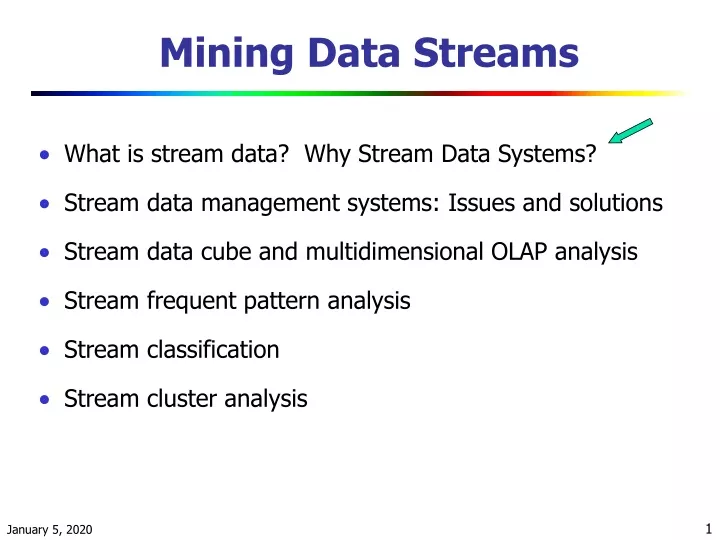
Mining Data Streams • What is stream data? Why Stream Data Systems? • Stream data management systems: Issues and solutions • Stream data cube and multidimensional OLAP analysis • Stream frequent pattern analysis • Stream classification • Stream cluster analysis
Mining Stream, Time-Series, and Sequence Data • Mining data streams • Mining time-series data • Mining sequence patterns in transactional databases • Mining sequence patterns in biological data
Characteristics of Data Streams • Data Streams • Data streams—continuous, ordered, changing, fast, huge amount • Traditional DBMS—data stored in finite, persistentdata sets • Characteristics • Huge volumes of continuous data, possibly infinite • Fast changing and requires fast, real-time response • Data stream captures nicely our data processing needs of today • Random access is expensive—single scan algorithm (can only have one look) • Store only the summary of the data seen thus far • Most stream data are at pretty low-level or multi-dimensional in nature, needs multi-level and multi-dimensional processing
Stream Data Applications • Telecommunication calling records • Business: credit card transaction flows • Network monitoring and traffic engineering • Financial market: stock exchange • Engineering & industrial processes: power supply & manufacturing • Sensor, monitoring & surveillance: video streams, RFIDs • Security monitoring • Web logs and Web page click streams • Massive data sets (even saved but random access is too expensive)
Persistent relations One-time queries Random access “Unbounded” disk store Only current state matters No real-time services Relatively low update rate Data at any granularity Assume precise data Access plan determined by query processor, physical DB design Transient streams Continuous queries Sequential access Bounded main memory Historical data is important Real-time requirements Possibly multi-GB arrival rate Data at fine granularity Data stale/imprecise Unpredictable/variable data arrival and characteristics DBMS versus DSMS Ack. From Motwani’s PODS tutorial slides
Mining Data Streams • What is stream data? Why Stream Data Systems? • Stream data management systems: Issues and solutions • Stream data cube and multidimensional OLAP analysis • Stream frequent pattern analysis • Stream classification • Stream cluster analysis
Continuous Query Architecture: Stream Query Processing SDMS (Stream Data Management System) User/Application Results Multiple streams Stream Query Processor Scratch Space (Main memory and/or Disk)
Challenges of Stream Data Processing • Multiple, continuous, rapid, time-varying, ordered streams • Main memory computations • Queries are often continuous • Evaluated continuously as stream data arrives • Answer updated over time • Queries are often complex • Beyond element-at-a-time processing • Beyond stream-at-a-time processing • Beyond relational queries (scientific, data mining, OLAP) • Multi-level/multi-dimensional processing and data mining • Most stream data are at low-level or multi-dimensional in nature
Processing Stream Queries • Query types • One-time query vs. continuous query (being evaluated continuously as stream continues to arrive) • Predefined query vs. ad-hoc query (issued on-line) • Unbounded memory requirements • For real-time response, main memory algorithm should be used • Memory requirement is unbounded if one will join future tuples • Approximate query answering • With bounded memory, it is not always possible to produce exact answers • High-quality approximate answers are desired • Data reduction and synopsis construction methods • Sketches, random sampling, histograms, wavelets, etc.
Methodologies for Stream Data Processing • Major challenges • Keep track of a large universe, e.g., pairs of IP address, not ages • Methodology • Synopses (trade-off between accuracy and storage) • Use synopsis data structure, much smaller (O(logk N) space) than their base data set (O(N) space) • Compute an approximate answer within a small error range (factor ε of the actual answer) • Major methods • Random sampling • Histograms • Sliding windows • Multi-resolution model • Sketches • Radomized algorithms
Stream Data Processing Methods (1) • Random sampling (but without knowing the total length in advance) • Reservoir sampling: maintain a set of s candidates in the reservoir, which form a true random sample of the element seen so far in the stream. As the data stream flow, every new element has a certain probability (s/N) of replacing an old element in the reservoir. • Sliding windows • Make decisions based only on recent data of sliding window size w • An element arriving at time t expires at time t + w • Histograms • Approximate the frequency distribution of element values in a stream • Partition data into a set of contiguous buckets • Equal-width (equal value range for buckets) vs. V-optimal (minimizing frequency variance within each bucket) • Multi-resolution models • Popular models: balanced binary trees, micro-clusters, and wavelets
Stream Data Processing Methods (2) • Sketches • Histograms and wavelets require multi-passes over the data but sketches can operate in a single pass • Frequency moments of a stream A = {a1, …, aN}, Fk: where v: the universe or domain size, mi: the frequency of i in the sequence • Given N elts and v values, sketches can approximate F0, F1, F2 in O(log v + log N) space • Randomized algorithms • Monte Carlo algorithm: bound on running time but may not return correct result • Chebyshev’s inequality: • Let X be a random variable with mean μ and standard deviation σ • Chernoff bound: • Let X be the sum of independent Poisson trials X1, …, Xn, δ in (0, 1] • The probability decreases expoentially as we move from the mean
Approximate Query Answering in Streams • Sliding windows • Only over sliding windows of recent stream data • Approximation but often more desirable in applications • Batched processing, sampling and synopses • Batched if update is fast but computing is slow • Compute periodically, not very timely • Sampling if update is slow but computing is fast • Compute using sample data, but not good for joins, etc. • Synopsis data structures • Maintain a small synopsis or sketch of data • Good for querying historical data • Blocking operators, e.g., sorting, avg, min, etc. • Blocking if unable to produce the first output until seeing the entire input
Stream Data Mining vs. Stream Querying • Stream mining—A more challenging task in many cases • It shares most of the difficulties with stream querying • But often requires less “precision”, e.g., no join, grouping, sorting • Patterns are hidden and more general than querying • It may require exploratory analysis • Not necessarily continuous queries • Stream data mining tasks • Multi-dimensional on-line analysis of streams • Mining outliers and unusual patterns in stream data • Clustering data streams • Classification of stream data
Mining Data Streams • What is stream data? Why Stream Data Systems? • Stream data management systems: Issues and solutions • Stream data cube and multidimensional OLAP analysis • Stream frequent pattern analysis • Stream classification • Stream cluster analysis
Challenges for Mining Dynamics in Data Streams • Most stream data are at pretty low-level or multi-dimensional in nature: needs ML/MD processing • Analysis requirements • Multi-dimensional trends and unusual patterns • Capturing important changes at multi-dimensions/levels • Fast, real-time detection and response • Comparing with data cube: Similarity and differences • Stream (data) cube or stream OLAP: Is this feasible? • Can we implement it efficiently?
Multi-Dimensional Stream Analysis: Examples • Analysis of Web click streams • Raw data at low levels: seconds, web page addresses, user IP addresses, … • Analysts want: changes, trends, unusual patterns, at reasonable levels of details • E.g., Average clicking traffic in North America on sports in the last 15 minutes is 40% higher than that in the last 24 hours.” • Analysis of power consumption streams • Raw data: power consumption flow for every household, every minute • Patterns one may find: average hourly power consumption surges up 30% for manufacturing companies in Chicago in the last 2 hours today than that of the same day a week ago
A Stream Cube Architecture • Atilted time frame • Different time granularities • second, minute, quarter, hour, day, week, … • Critical layers • Minimum interest layer (m-layer) • Observation layer (o-layer) • User: watches at o-layer and occasionally needs to drill-down down to m-layer • Partial materialization of stream cubes • Full materialization: too space and time consuming • No materialization: slow response at query time • Partial materialization: what do we mean “partial”?
A Titled Time Model • Natural tilted time frame: • Example: Minimal: quarter, then 4 quarters 1 hour, 24 hours day, … • Logarithmic tilted time frame: • Example: Minimal: 1 minute, then 1, 2, 4, 8, 16, 32, …
A Titled Time Model (2) • Pyramidal tilted time frame: • Example: Suppose there are 5 frames and each takes maximal 3 snapshots • Given a snapshot number N, if N mod 2d = 0, insert into the frame number d. If there are more than 3 snapshots, “kick out” the oldest one.
Two Critical Layers in the Stream Cube (*, theme, quarter) o-layer (observation) (user-group, URL-group, minute) m-layer (minimal interest) (individual-user, URL, second) (primitive) stream data layer
On-Line Partial Materialization vs. OLAP Processing • On-line materialization • Materialization takes precious space and time • Only incremental materialization (with tilted time frame) • Only materialize “cuboids” of the critical layers? • Online computation may take too much time • Preferred solution: • popular-path approach: Materializing those along the popular drilling paths • H-tree structure: Such cuboids can be computed and stored efficiently using the H-tree structure • Online aggregation vs. query-based computation • Online computing while streaming: aggregating stream cubes • Query-based computation: using computed cuboids
root Observation layer Urbana Springfield Chicago .gov .com .com .edu Elec Bio Elec Chem 6:00AM-7:00AM 156 7:00AM-8:00AM 201 8:00AM-9:00AM 235 …… An H-Tree Cubing Structure Minimal int. layer
Benefits of H-Tree and H-Cubing • H-tree and H-cubing • Developed for computing data cubes and ice-berg cubes • J. Han, J. Pei, G. Dong, and K. Wang, “Efficient Computation of Iceberg Cubes with Complex Measures”, SIGMOD'01 • Fast cubing, space preserving in cube computation • Using H-tree for stream cubing • Space preserving • Intermediate aggregates can be computed incrementally and saved in tree nodes • Facilitate computing other cells and multi-dimensional analysis • H-tree with computed cells can be viewed as stream cube
Mining Data Streams • What is stream data? Why Stream Data Systems? • Stream data management systems: Issues and solutions • Stream data cube and multidimensional OLAP analysis • Stream frequent pattern analysis • Stream classification • Stream cluster analysis
Frequent Patterns for Stream Data • Frequent pattern mining is valuable in stream applications • e.g., network intrusion mining (Dokas, et al’02) • Mining precise freq. patterns in stream data: unrealistic • Even store them in a compressed form, such as FPtree • How to mine frequent patterns with good approximation? • Approximate frequent patterns (Manku & Motwani VLDB’02) • Keep only current frequent patterns? No changes can be detected • Mining evolution freq. patterns (C. Giannella, J. Han, X. Yan, P.S. Yu, 2003) • Use tilted time window frame • Mining evolution and dramatic changes of frequent patterns • Space-saving computation of frequent and top-k elements (Metwally, Agrawal, and El Abbadi, ICDT'05)
Mining Approximate Frequent Patterns • Mining precise freq. patterns in stream data: unrealistic • Even store them in a compressed form, such as FPtree • Approximate answers are often sufficient (e.g., trend/pattern analysis) • Example: a router is interested in all flows: • whose frequency is at least 1% (σ) of the entire traffic stream seen so far • and feels that 1/10 of σ (ε= 0.1%) error is comfortable • How to mine frequent patterns with good approximation? • Lossy Counting Algorithm (Manku & Motwani, VLDB’02) • Major ideas: not tracing items until it becomes frequent • Adv: guaranteed error bound • Disadv: keep a large set of traces
Bucket 1 Bucket 2 Bucket 3 Lossy Counting for Frequent Items Divide Stream into ‘Buckets’ (bucket size is 1/ ε = 1000)
Empty (summary) + At bucket boundary, decrease all counters by 1 First Bucket of Stream
+ At bucket boundary, decrease all counters by 1 Next Bucket of Stream
Approximation Guarantee • Given: (1) support threshold: σ, (2) error threshold: ε, and (3) stream length N • Output: items with frequency counts exceeding (σ–ε) N • How much do we undercount? If stream length seen so far = N and bucket-size = 1/ε then frequency count error #buckets = εN • Approximation guarantee • No false negatives • False positives have true frequency count at least (σ–ε)N • Frequency count underestimated by at most εN
Bucket 1 Bucket 2 Bucket 3 Lossy Counting For Frequent Itemsets Divide Stream into ‘Buckets’ as for frequent items But fill as many buckets as possible in main memory one time If we put 3 buckets of data into main memory one time, Then decrease each frequency count by 3
2 2 4 3 1 4 3 2 10 1 2 + 9 1 2 1 0 3 bucket data in memory summary data Update of Summary Data Structure summary data Itemset ( ) is deleted.That’s why we choose a large number of buckets – delete more
1 2 Pruning Itemsets – Apriori Rule 2 + 1 1 3 bucket data in memory summary data If we find itemset ( ) is not frequent itemset, Then we needn’t consider its superset
Summary of Lossy Counting • Strength • A simple idea • Can be extended to frequent itemsets • Weakness: • Space Bound is not good • For frequent itemsets, they do scan each record many times • The output is based on all previous data. But sometimes, we are only interested in recent data • A space-saving method for stream frequent item mining • Metwally, Agrawal and El Abbadi, ICDT'05
Mining Evolution of Frequent Patterns for Stream Data • Approximate frequent patterns (Manku & Motwani VLDB’02) • Keep only current frequent patterns—No changes can be detected • Mining evolution and dramatic changes of frequent patterns (Giannella, Han, Yan, Yu, 2003) • Use tilted time window frame • Use compressed form to store significant (approximate) frequent patterns and their time-dependent traces • Note: To mine precise counts, one has to trace/keep a fixed (and small) set of items
Two Structures for Mining Frequent Patterns with Tilted-Time Window • FP-Trees store Frequent Patterns, rather than Transactions • Tilted-time major: An FP-tree for each tilted time frame
Frequent Pattern & Tilted-Time Window (2) • The second data structure: • Observation: FP-Trees of different time units are similar • Pattern-tree major: each node is associated with a tilted-time window
Mining Data Streams • What is stream data? Why Stream Data Systems? • Stream data management systems: Issues and solutions • Stream data cube and multidimensional OLAP analysis • Stream frequent pattern analysis • Stream classification • Stream cluster analysis
Classification for Dynamic Data Streams • Decision tree induction for stream data classification • VFDT (Very Fast Decision Tree)/CVFDT (Domingos, Hulten, Spencer, KDD00/KDD01) • Is decision-tree good for modeling fast changing data, e.g., stock market analysis? • Other stream classification methods • Instead of decision-trees, consider other models • Naïve Bayesian • Ensemble (Wang, Fan, Yu, Han. KDD’03) • K-nearest neighbors (Aggarwal, Han, Wang, Yu. KDD’04) • Tilted time framework, incremental updating, dynamic maintenance, and model construction • Comparing of models to find changes
Hoeffding Tree • With high probability, classifies tuples the same • Only uses small sample • Based on Hoeffding Bound principle • Hoeffding Bound (Additive Chernoff Bound) r: random variable R: range of r n: # independent observations Mean of r is at least ravg – ε, with probability 1 – d
Hoeffding Tree Algorithm • Hoeffding Tree Input S: sequence of examples X: attributes G( ): evaluation function d: desired accuracy • Hoeffding Tree Algorithm for each example in S retrieve G(Xa) and G(Xb) //two highest G(Xi) if ( G(Xa) – G(Xb) > ε ) split on Xa recurse to next node break
Decision-Tree Induction with Data Streams Packets > 10 Data Stream yes no Protocol = http Packets > 10 Data Stream yes no Bytes > 60K Protocol = http yes Protocol = ftp Ack. From Gehrke’s SIGMOD tutorial slides
Hoeffding Tree: Strengths and Weaknesses • Strengths • Scales better than traditional methods • Sublinear with sampling • Very small memory utilization • Incremental • Make class predictions in parallel • New examples are added as they come • Weakness • Could spend a lot of time with ties • Memory used with tree expansion • Number of candidate attributes
VFDT (Very Fast Decision Tree) • Modifications to Hoeffding Tree • Near-ties broken more aggressively • G computed every nmin • Deactivates certain leaves to save memory • Poor attributes dropped • Initialize with traditional learner (helps learning curve) • Compare to Hoeffding Tree: Better time and memory • Compare to traditional decision tree • Similar accuracy • Better runtime with 1.61 million examples • 21 minutes for VFDT • 24 hours for C4.5 • Still does not handle concept drift
CVFDT (Concept-adapting VFDT) • Concept Drift • Time-changing data streams • Incorporate new and eliminate old • CVFDT • Increments count with new example • Decrement old example • Sliding window • Nodes assigned monotonically increasing IDs • Grows alternate subtrees • When alternate more accurate => replace old • O(w) better runtime than VFDT-window
Ensemble of Classifiers Algorithm • H. Wang, W. Fan, P. S. Yu, and J. Han, “Mining Concept-Drifting Data Streams using Ensemble Classifiers”, KDD'03. • Method (derived from the ensemble idea in classification) • train K classifiers from K chunks • for each subsequent chunk train a new classifier test other classifiers against the chunk assign weight to each classifier select top K classifiers
Mining Data Streams • What is stream data? Why Stream Data Systems? • Stream data management systems: Issues and solutions • Stream data cube and multidimensional OLAP analysis • Stream frequent pattern analysis • Stream classification • Stream cluster analysis
Clustering Data Streams [GMMO01] • Base on the k-median method • Data stream points from metric space • Find k clusters in the stream s.t. the sum of distances from data points to their closest center is minimized • Constant factor approximation algorithm • In small space, a simple two step algorithm: • For each set of M records, Si, find O(k) centers in S1, …, Sl • Local clustering: Assign each point in Si to its closest center • Let S’ be centers for S1, …, Sl with each center weighted by number of points assigned to it • Cluster S’ to find k centers