Download
1 / 38
380 likes | 491 Views
ASSOCIATION. Association The strength of relationship between 2 variables Knowing how much variables are related may enable you to predict the value of 1 variable when you know the value of another Practical significance vs. statistical significance

E N D
ASSOCIATION • Association • The strength of relationship between 2 variables • Knowing how much variables are related may enable you to predict the value of 1 variable when you know the value of another • Practical significance vs. statistical significance • Statistically significant does not mean strong, or meaningful
Review for Nominal or Nominal-Ordinal Combinations • 2 based measures • 2 captures the strength of a relationship but also N. To get a “pure” measure of strength, you have to remove influence of N • Phi • Cramer's V • PRE measures • Improvement in prediction you get by knowing the IV (or reduction in error) • Lambda
2 LIMITATIONS OF LAMBDA 1. Asymmetric • Value of the statistic will vary depending on which variable is taken as independent 2. Misleading when one of the row totals is much larger than the other(s) • For this reason, when row totals are extremely uneven, use a chi square-based measure instead
MEASURE OF ASSOCIATION—BOTH VARIABLES ORDINAL • GAMMA • For examining STRENGTH & DIRECTION of “collapsed” ordinal variables (<6 categories) • Like Lambda, a PRE-based measure • Range is -1.0 to +1.0
GAMMA • Logic: Applying PRE to PAIRS of individuals
GAMMA • CONSIDER KENNY-DEB PAIR • In the language of Gamma, this is a “same” pair • direction of difference on 1 variable is the same as direction on the other • If you focused on the Kenny-Eric pair, you would come to the same conclusion
GAMMA • NOW LOOK AT THE TIM-JOEY PAIR • In the language of Gamma, this is a “different” pair • direction of difference on one variable is opposite of the difference on the other
GAMMA • Logic: Applying PRE to PAIRS of individuals • Formula: same – different same + different
GAMMA • If you were to account for all the pairs in this table, you would find that there were 9 “same” & 9 “different” pairs • Applying the Gamma formula, we would get: 9 – 9 = 0 = 0.0 18 18
GAMMA • 3-case example • Applying the Gamma formula, we would get: 3 – 0 = 3 = 1.00 3 3
Gamma: Example 1 • Examining the relationship between: • FEHELP (“Wife should help husband’s career first”) & • FEFAM (“Better for man to work, women to tend home”) • Both variables are ordinal, coded 1 (strongly agree) to 4 (strongly disagree)
Gamma: Example 1 • Based on the info in this table, does there seem to be a relationship between these factors? • Does there seem to be a positive or negative relationship between them? • Does this appear to be a strong or weak relationship?
GAMMA • Do we reject the null hypothesis of independence between these 2 variables? • Yes, the Pearson chi square p value (.000) is < alpha (.05) • It’s worthwhile to look at gamma. • Interpretation: • There is a strong positive relationship between these factors. • Knowing someone’s view on a wife’s “first priority” improves our ability to predict whether they agree that women should tend home by 75.5%.
USING GSS DATA • Construct a contingency table using two ordinal level variables • Are the two variables significantly related? • How strong is the relationship? • What direction is the relationship?
Scattergrams • Allow quick identification of important features of relationship between interval-ratio variables • Two dimensions: • Scores of the independent (X) variable (horizontal axis) • Scores of the dependent (Y) variable (vertical axis)
3 Purposes of Scattergrams • To give a rough idea about the existence, strength & direction of a relationship • The direction of the relationship can be detected by the angle of the regression line 2. To give a rough idea about whether a relationship between 2 variables is linear (defined with a straight line) 3. To predict scores of cases on one variable (Y) from the score on the other (X)
IV and DV? • What is the direction • of this relationship?
IV and DV? • What is the direction of this relationship?
The Regression line • Properties: • The sum of positive and negative vertical distances from it is zero • The standard deviation of the points from the line is at a minimum • The line passes through the point (mean x, mean y) • Bivariate Regression Applet
Regression Line Formula Y = a + bX Y = score on the dependent variable X = the score on the independent variable a = the Y intercept – point where the regression line crosses the Y axis b = the slope of the regression line • SLOPE – the amount of change produced in Y by a unit change in X; or, • a measure of the effect of the X variable on the Y
Regression Line Formula Y = a + bX y-intercept (a) = 102 slope (b) = .9 Y = 102 + (.9)X • This information can be used to predict weight from height. • Example: What is the predicted weight of a male who is 70” tall (5’10”)? • Y = 102 + (.9)(70) = 102 + 63 = 165 pounds
Example 2: Examining the link between # hours of daily TV watching (X) & # of cans of soda consumed per day (Y)
Example 2 • Example 2: Examining the link between # hours of daily TV watching (X) & # of cans of soda consumed per day. (Y) • The regression line for this problem: • Y = 0.7 + .99x • If a person watches 3 hours of TV per day, how many cans of soda would he be expected to consume according to the regression equation?
The Slope (b) – A Strength & A Weakness • We know that b indicates the change in Y for a unit change in X, but b is not really a good measure of strength • Weakness • It is unbounded (can be >1 or <-1) making it hard to interpret • The size of b is influenced by the scale that each variable is measured on
Pearson’s r Correlation Coefficient • By contrast, Pearson’s r is bounded • a value of 0.0 indicates no linear relationship and a value of +/-1.00 indicates a perfect linear relationship
Pearson’s r Y = 0.7 + .99x sx = 1.51 sy = 2.24 • Converting the slope to a Pearson’s r correlation coefficient: • Formula: r = b(sx/sy) r = .99 (1.51/2.24) r = .67
The Coefficient of Determination • The interpretation of Pearson’s r (like Cramer’s V) is not straightforward • What is a “strong” or “weak” correlation? • Subjective • The coefficient of determination (r2) is a more direct way to interpret the association between 2 variables • r2 represents the amount of variation in Y explained by X • You can interpret r2 with PRE logic: • predict Y while ignoring info. supplied by X • then account for X when predicting Y
Coefficient of Determination: Example • Without info about X (hours of daily TV watching), the best predictor we have is the mean # of cans of soda consumed (mean of Y) • The green line (the slope) is what we would predict WITH info about X
Coefficient of Determination • Conceptually, the formula for r2 is: r2 = Explained variation Total variation “The proportion of the total variation in Y that is attributable or explained by X.” • The variation not explained by r2 is called the unexplained variation • Usually attributed to measurement error, random chance, or some combination of other variables
Coefficient of Determination • Interpreting the meaning of the coefficient of determination in the example: • Squaring Pearson’s r (.67) gives us an r2 of .45 • Interpretation: • The # of hours of daily TV watching (X) explains 45% of the total variation in soda consumed (Y)
Another Example: Relationship between Mobility Rate (x) & Divorce rate (y) • The formula for this regression line is: Y = -2.5 + (.17)X • 1) What is this slope telling you? • 2) Using this formula, if the mobility rate for a given state was 45, what would you predict the divorce rate to be? • 3) The standard deviation (s) for x=6.57 & the s for y=1.29. Use this info to calculate Pearson’s r. How would you interpret this correlation? • 4) Calculate & interpret the coefficient of determination (r2)
Another Example: Relationship between Mobility Rate (x) & Divorce rate (y) • The formula for this regression line is: Y = -2.5 + (.17)X • 1) What is this slope telling you? • 2) Using this formula, if the mobility rate for a given state was 45, what would you predict the divorce rate to be? • 3) The standard deviation (s) for x=6.57 & the s for y=1.29. Use this info to calculate Pearson’s r. How would you interpret this correlation? • 4) Calculate & interpret the coefficient of determination (r2)
Regression Output • Scatterplot • Graphs Legacy Simple Scatter • Regression • Analyze Regression Linear • Example: How much you work predicts how much time you have to relax • X = Hours worked in past week • Y = Hours relaxed in past week
Correlation Matrix • Analyze Correlate Bivariate
Measures of Association * But, has an upper limit of 1 when dealing with a 2x2 table.