Download
1 / 39
390 likes | 480 Views
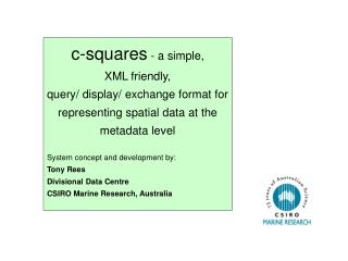
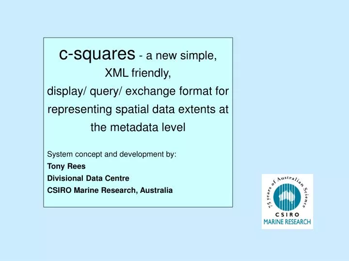
c-squares - a new simple, XML friendly, display/ query/ exchange format for representing spatial data extents at the metadata level System concept and development by: Tony Rees Divisional Data Centre CSIRO Marine Research, Australia. Topics to be covered.

E N D
c-squares - a new simple, XML friendly, display/ query/ exchange format for representing spatial data extents at the metadata level System concept and development by: Tony Rees Divisional Data Centre CSIRO Marine Research, Australia
Topics to be covered ... • Characteristics of metadata, and metadata spatial searches • Problems with “bounding rectangles” as representations of dataset extents • The c-squares concept • c-squares in practice • Future possibilities
Metadata records (structured dataset descriptions) - as text files, database, or XML format metadata query and/or exchange (Metadata level) dataset descriptions in standard format The Metadata concept ... (Data level) Data Store 1 Data Store 2 offline digital data databases / data warehouses offline nondigital data
some example Metadatabases (Data Directories) ... + many others -- 100 < 1000? ... • Metadata records exist independently of the datasets they describe, may not necessarily have on-line connection to the actual data --- i.e., they act as surrogates for the data • Spatial searching (where implemented) typically by bounding rectangles (N,S,W,E limits) or sometimes defined regions (R1 yes/no, R2 yes/no, etc.)
“Bounding rectangles” test: if search rectangle (blue) overlaps data rectangle (red), a supposed “hit” is returned : false hit no hit hit current “first pass” representation of spatial data coverage is by bounding coordinates - example: <metadata> <title>Franklin Voyage FR 10/87 CTD Data</title> <custodianOrg>CSIRO Marine Research</custodianOrg> (etc. etc.) <boundingBox> <northBoundingCoord>-9.0</northBoundingCoord> <southBoundingCoord>-19.0</southBoundingCoord> <westBoundingCoord>117.0</westBoundingCoord> <eastBoundingCoord>145.8</eastBoundingCoord> </boundingBox> (etc. etc.) • concept introduced in FGDC draft metadata standard, 1994 • used for distributed spatial searching, 1995 onwards • still the primary tool for conducting metadata spatial searches; integral to ISO 19115 draft metadata standard, 2002 • polygons are also enterable, but seldom used for searching owing to the arithmetic overhead involved
Bounding coordinates - pluses and minuses • Pluses ... • Metadata elements are concise • User-entry is simple • Spatial searching is simple arithmetic operation (looks for overlap between a “search” rectangle and available “data” rectangles) • Useful as a “first pass” -- rapidly filters out many datasets not close to the region of interest • Minuses … • A rectangular shape does not correspond to the actual shape of many datasets • Data distribution may be aligned along other than N-S or E-W axes • Data distribution may be patchy or incomplete within the designated boundary • Corollary … Apparent “hits” never 100% reliable (unless the data are always rectangular, e.g. mapsheets)
Some real-world examples (other agencies’ data) ...
our agency’s data (marine surveys) - examples ... NB, “bounding rectangle” searches result in many false or misleading hits, since large portions of the “dataset” rectangles contain no data - particularly where surveys wrap around a feature or land area, or are oriented obliquely with respect to N-S, or E-W directions.
Germ of c-squares concept ... from Ken Walker’s Bioinformatics search interface, Museum Victoria (Australia) • state divided into 0.5 x 0.5 º squares (numbered as per relevant mapsheets) • search interface has direct connection to base data (>100,000 point data records) • each base data record is tagged with its relevant mapsheet number, so spatial searching is by simple numeric/text match (no arithmetic required) • user can request list of hits (species) from one or multiple search squares (e.g. blue hatched examples) 700 km
modifications which would be required for use with metadata ... • multiple square id’s could be stored in single metadata record (harvested from base data) - removes requirement to access the base data to answer search queries • numbering system should be expanded to become globally applicable • geographic scale (size of squares) should be variable up or down to suit variety of user needs • metadata records become storage vehicles for dataset “footprints” (simple spatial objects) 700 km
The “c-squares” concept c-squares: Concise Spatial Query and Representation System
data “footprint” using 1 x 1 degree c-squares same using 0.5 x 0.5 degree c-squares “c-squares” principle • “c-squares string” holds ID’s of all the tiles (e.g. 1 x 1, 0.5 x 0.5 degree squares) which are intersected by the dataset spatial extent (footprint) actual survey location - “Franklin” cruise 10/87 data “footprint” using bounding rectangle
“c-squares” numbering system • each square is numbered according to a globally applicable system based on recursive divisions of WMO (World Meteorological organisation) 10-degree squares, e.g.: • 10 degree square: 3414(= WMO number) • 5 degree square: 3414:2 • 1 degree square: 3414:227 • 0.5 degree square: 3414:227:4 • 0.1 degree square: 3414:227:466 • (etc.) • strings of codes represent an individual dataset extent, e.g. • 3013:497|3111:468|3111:478|3111:479|3111:488|3111:489|3111:499|3112:122|3112:123| • 3112:131|3112:132|3112:134|3112:141|3112:142|3112:143|3112:217|3112:218|3112:219| • 3112:226|3112:235|3112:350|3112:351|3112:352|3112:353|3112:360|3112:361|3112:362| • 3112:363|3112:370|3112:371|3112:380|3112:381|3112:390|3113:100|3113:101|3113:102| • 3113:103|3113:104|3113:205|3113:206|3113:207|3113:216|3113:217|3113:228|3113:238| • 3113:239 • encodes the extent • shown in the example:
WMO 10-degree squares notation (part) (Available via the web in NODC, 1998:World Ocean Database 1998 Documentation)
WMO 10-degree squares notation principle NE sector (1xxx) 7800 NW sector (7xxx) 7017 7000 1017 5017 5000 3000 3017 SW sector (5xxx) SE sector (3xxx) 5800 3800
nomenclature for 5-degree squares - e.g. in SE sector: • follows “Blue Pages” (1996) extension of WMO numbering, using 4 quadrants (1, 2, 3, 4) for 5-degree squares - e.g. within 10-degree square 3414 ... 140 145 150 -40 WMO 10-degree square 3414 (grey) 5-degree square 3414:2 (light blue) 1 2 -45 4 3 3414 -50 (1 is always closest to global origin, 4 is always furthest away. For full specification refer c-squares website)
nomenclature for 1-degree squares - e.g. in SE sector: • follows “Blue Pages” (1996) extension of WMO numbering, using 4 quadrants (1, 2, 3, 4) for 5-degree squares, plus 2 digits 00-99 for 1-degree squares - e.g. within 10-degree square 3414 ... 140 145 150 -40 100 101 102 103 104 205 206 207 208 209 WMO 10-degree square 3414 (grey) 5-degree square 3414:2 (light blue) 1-degree square 3414:227 (green) 110 111 112 113 114 215 216 217 218 219 120 121 122 123 124 225 226 227 228 229 238 130 131 132 133 134 235 236 237 239 140 141 142 143 144 245 246 247 248 249 -45 350 351 352 353 354 455 456 457 458 449 360 361 362 363 364 465 466 467 468 469 370 371 372 373 374 475 476 477 478 479 380 381 382 383 384 485 486 487 488 3414 489 390 391 392 393 394 495 496 497 498 499 -50 (100 is always closest to global origin, 499 is always furthest away. For full specification refer c-squares website)
Codes have straightforward relationship with lats/longs, mapsheets, etc. ... e.g.: 3414:227(1-degree square with origin at 42 ºS, 147 ºE) additional degrees E [140+7] =147 additional degrees S [40+2] = 42 5-degree quadrant, i.e. 1 2 3 4 tens of degrees E (i.e., 140) tens of degrees S (i.e., 40) global sector (1=NE, 3=SE, 5=SW, 7=NW) 70 km
“quad tree” -type approach used where numerous adjacent squares are occupied example: 3212:*** can be used instead of specifying every 1-degree square within 10 degree square 3212. This leads to corresponding data reduction, e.g. Australia (at 1-degree resolution) can be described in 343 squares rather than 800:
Example database-level implementation of c-squares for metadata records(e.g. at 1 degree resolution) (etc.)
3315:131:1 3315:130:2 3315:130:1 3315:131:3 3315:130:4 3315:130:3 Options for c-squares data entry ... • automated conversion of lat/long data to c-squares (ignoring multiple hits) • automated conversion of GIS polygon data to c-squares extents • clickable map interface for region(s) of immediate interest • manual entry, with reference to marked-up mapsheet/s • on-line lat/long - to - c-square converter • custom digitising system (graphics tablet data input or similar) clickable map interface (generalised example) mapsheet marked with 0.5 degree squares - for manual entry
Process invoked for web mapping (1) c-squares strings can be transformed into coordinate pairs (centre point of squares) and square size, by an appropriate function and then sent to Xerox PARC Map Viewer or similar, e.g.:
Process invoked for web mapping (2) c-squares strings can be sent directly to the CMR c-squares mapper (accessible via the web), e.g.:
Further examples (CMR oceanographic/biological data - 0.5 x 0.5 deg. squares): (Base maps are automatically chosen to fit the data range, or can be selected manually)
Mechanism for spatial queries using c-squares • c-squares spatial queries simply test whether a text string representing the search box (ideally one or several c-squares) is matched anywhere in the c-squares string … • example: - search square 3113:2 will match any c-squares string which includes 3113:2 within it, e.g.: • <csquares> • 3013:497|3111:468|3111:478|3111:479|3111:488|3111:489|3111:499|3112:122|3112:123| • 3112:131|3112:132|3112:134|3112:141|3112:142|3112:143|3112:217|3112:218|3112:219| • 3112:226|3112:235|3112:350|3112:351|3112:352|3112:353|3112:360|3112:361|3112:362| • 3112:363|3112:370|3112:371|3112:380|3112:381|3112:390|3113:100|3113:101|3113:102| • 3113:103|3113:104|3113:205|3113:206|3113:207|3113:216|3113:217|3113:228|3113:238| • 3113:239 • </csquares> • (NB, this is a simple text search and involves no arithmetic - cf. querying of bounding rectangles, polygons, or more complex spatial objects) • hierarchical naming system for c-squares means that finer resolution squares are automatically picked up in any “coarser resolution” search
Implementable as a simple “click on a square” interface, e.g.:
… system does the search - checks for c-squares match if available (provides reliable matches), otherwise uses overlapping rectangles test (“possible match”) ...
produces ... (etc.)
Viewing the full metadata record produces ... with clickable link to show dataset extent using c-squares: (etc.)
Base maps for displayed data can be changed at will by the user, e.g.: (numerous other maps available, sample only shown)
c-squares strings are suitable for inclusion as a new XML metadata element, for example ... <metadata> <title>Franklin Voyage FR 10/87 CTD Data</title> <custodianOrg>CSIRO Marine Research</custodianOrg> (etc. etc.) <boundingBox> <northBoundingCoord>-9.0</northBoundingCoord> <southBoundingCoord>-19.0</southBoundingCoord> <westBoundingCoord>117.0</westBoundingCoord> <eastBoundingCoord>145.8</eastBoundingCoord> </boundingBox> <csquares>3111:499:2|3112:390:1|3111:489:3|3112:380:3|3112:380:4|3112:381:1|3111:488:2|3112:381:2|3112:371:3|3111:478:4|3112:370:4|3112:370:1|3111:478:1|3111:479:2|3111:479:1|3112:361:4|3111:468:4|3112:363:3|3112:361:3|3111:467:2|3112:360:2|3112:363:1|3112:362:2|3112:360:1|3112:352:4|3112:352:3|3112:350:4|3112:352:1|3112:351:2|3112:352:2|3112:353:2|3112:353:1</csquares> </metadata>
Actual size of c-squares, e.g. compared to U.K. : WMO Square7500 7500 1000 x 600 km 10 x 10 deg. 7500:1 500 x 300 km 5 x 5 deg. 1 x 1 deg. 7500:123 100 x 60 km 0.5 x 0.5 deg. 7500:123:4 50 x 30 km 0.1 x 0.1 deg. 7500:123:455 10 x 6 km (NB, “real” shape and dimensions vary according to position on globe) • 1 x 1 degree squares is suggested as a possible minimum standard of spatial encoding for global interoperability of metadata systems (finer resolution available to users on as-needs basis)
Summary - strengths and weaknesses of c-squares • Strengths ... • “c-squares” metadata element is a concise and flexible way of encoding a wide variety of different spatial objects - including nonlinear and incomplete (patchy) coverages • automated or manual code entry (and maintenance) is possible, and relatively simple • spatial searching is simple text string matching operation -- no supporting GIS system is required ( i.e., zero technological overhead) • “c-squares mapper” utility provides rapid and flexible data extent visualisations, and can be called from anywhere via the web • can be implemented progressively into any metadata system as an adjunct to bounding coordinates (a search can be configured to work with whatever is available) • Weaknesses … • may not be the only numbering convention available (Marsden Squares and Maidenhead Locators are alternatives to WMO squares, however less suitable in this application) • c-squares are not uniform shape/size across the earth’s surface (true squares only at the equator); some local/national grids do not transform easily to lat/long squares • may be cumbersome to encode very large, complex regions (e.g. “Pacific Ocean”) by this method - works best at continental scales and below.
other comments ... • “c-squares” notation is language-independent - can be equally used in English, French, Japanese … also discipline-independent (suitable for physical, biological, geological, topographical, plus any other data type) • downwards-scalability of the c-squares notation means that it can be applied to any size region (e.g. local level) • equally applicable to terrestrial and marine data • no equivalent in GML notation at this time (GML only supports vector data). Even if there were a GML equivalent, c-squares would still be significantly more concise.
c-squares future ... • c-squares is being implemented progressively in CSIRO Marine Research’s “MarLIN” metadata system (c. 500 records to date, more continuously added) and in the CMR “CAAB” marine species dictionary (c. 3000 records). MarLIN c-squares search interface is already operational • c-squares is freely available for implementation in any other agencies’ metadata systems. Possibly small “islands of interoperability” could be created, or system could simply be implemented for within-agency use • c-squares could be offered to relevant user community/national bodies as an optional metadata element - possibly as a user-defined extension to a recognised metadata standard (e.g. ANZLIC, ISO) • current CMR c-squares mapper is already accessible for general use. Global and selected regional mapping options already available and can be developed further. External systems already linking to the c-squares mapper include OBIS (Ocean Biogeographic Information System, USA) and FishBase (ICLARM/FAO), as well as CMR’s MarLIN and CAAB databases • c-squares website (www.marine.csiro.au/csquares/) is a focal point for all c-squares related materials - including specification, background information, sample code, on-line lat/long converter, sample c-squares-enabled metadata records, and more
Potential Implementation across multiple systems Single or multi catalogue query with c-squares Single or multi catalogue query with c-squares metadata query and/or exchange with c-squares + bounding rectangles catalogue 1 metadata query and/or exchange with bounding rectangles catalogue 2 (c-squares enabled - whole or part) (non c-squares enabled) Single or multi catalogue query with bounding rectangles catalogue 3
Acknowledgements/Inspiration ... • Ken Walker (Museum Victoria) for showing me his Museum Victoria Bioinformatics search interface, based on 0.5 degree squares • “Blue Pages” Marine and Coastal Data Directory (MCDD) for the notation for subdividing WMO squares, also for pointers to software for drawing rectangles on GIF images (as used in the c-squares mapper) and for point-and-click map searching • CMR Data Centre staff for useful feedback • Miroslaw Ryba (CMR) for programming assistance with the c-squares mapper • John Hockaday (Geoscience Australia) and Doug Nebert (FGDC, USA) for helpful comments on prototype versions of the system • NOAA “GLOBE” Project and Martin Dix, CSIRO Atmospheric Research for provision of backdrop images used in the c-squares mapper.