Download
1 / 35
350 likes | 483 Views
c-squares - a simple, XML friendly, query/ display/ exchange format for representing spatial data at the metadata level System concept and development by: Tony Rees Divisional Data Centre CSIRO Marine Research, Australia. examples of current metadata systems. new all-CSIRO directory.

E N D
c-squares - a simple, XML friendly, query/ display/ exchange format for representing spatial data at the metadata level System concept and development by: Tony Rees Divisional Data Centre CSIRO Marine Research, Australia
examples of current metadata systems ... new all-CSIRO directory OBIS, USA (planned)
Metadata versus Data Metadata records (text files, database, or XML format) (Metadata level) metadata query and/or exchange dataset descriptions in standard format (Data level) Data Store 1 Data Store 2 offline digital data databases / data warehouses offline nondigital data
Some Characteristics of Metadata • Normally a text (ASCII) file, divided into individual metadata fields (e.g. with XML markup or similar) • Can be searched as plain text (minimum) or, if stored in a database, by more sophisticated methods • Represents a level of abstraction from the actual data - documents the most useful summary information for potential users, including spatial aspects (e.g. bounding coordinates, location keywords) • Should function as a stand-alone “surrogate” for the data for discovery and appraisal purposes - frequently decoupled from the actual data (which may or may not be available on-line) • May have different distribution/access privileges from the actual data.
Current preferred metadata transfer format is XML (ASCII) file, e.g… (excerpt): <metadata> <title>Franklin Voyage FR 07/93 CTD Data</title> <custodianOrg>CSIRO Marine Research</custodianOrg> (etc. etc.) <boundingBox> <northBoundingCoord>-30.0</northBoundingCoord> <southBoundingCoord>-44.0</southBoundingCoord> <westBoundingCoord>147.0</westBoundingCoord> <eastBoundingCoord>173.0</eastBoundingCoord> </boundingBox> (etc. etc.) </metadata>
“standard” representation of spatial data coverage in a sample metadata record
actual data distribution for the preceding example (CTD data, Franklin voyage FR 07/93) NB, standard spatial searches (by intersecting or overlapping rectangles) will produce numerous false “hits” (erroneous values) since most of the bounding rectangle for this dataset is empty
Data coverage is not always rectangular - frequently fills a non-rectangular shape (b), follows an edge or contour (c), surrounds an object (e.g. island or continent), (d), is discontinuous (e), linear/oblique (f), or extremely patchy (g) (a) (b) (c) (d) (e) (f) (g)
Why searching using overlapping rectangles is fallible bounding rectangle specified for search bounding rectangle for dataset data coverage (a) (b) (c) (d) (e) (f) (g) - for data of types (b) - (g), many searches by overlapping rectangles will produce “false hits”
Further examples of real data (species distributions) Note, only one of these plots is at all well represented by its “bounding coordinates” box
“c-squares” solution • “c-squares” is a system for improved metadata representation of spatial data which supports reliable spatial queries and provides meaningful visual representations (footprints) of dataset spatial coverage. It is fully transparent, royalty free, and vendor/platform independent, and available for immediate use. • c-squares comprises the following elements: • a nested set of proposed “standard” spatial resolutions for dataset description (levels 1-3), with all metadata at level 1 potentially interoperable • a custom, scalable nomenclature for “base level” individual geosquares, building on established standards, in a simple human- and machine- readable format • a syntax for representing strings of such geosquares in an editable and transportable ASCII format, in particular for use within a XML or similar metadata records • algorithms for translating any geolocated data between lats/longs and c-square codes, and vice versa, and • simple connectivity to basic mapping packages, including “freeware” such as the online Xerox PARC mapper.
Data “footprint” using bounding coordinates (as held in a metadata record) Data “footprint” using c-squares (also in metadata record) Example ...
“c-squares” standard resolutions • c-squares level 1 (fully interoperable) operates at 0.5 x 0.5 degree spatial resolution, or some 50-70 kms point-to-point in most regions of the globe • c-squares levels 2 and 3 (locally interoperable where implemented by users) operate at 0.1 x 0.1 and 0.02 x 0.02 degree (around 10 and 2 kms, respectively) spatial resolution, for higher resolution spatial representation where needed • c-squares levels 4-unlimited are not formally defined, but can be implemented by users on an “as needs” basis by simple extension from c-squares level 3. • Examples: c-squares level 1 code: SI5605f (0.5 x 0.5 deg. square) • c-squares level 2 code: SI5605fa (0.1 x 0.1 deg. square) • c-squares level 3 code: SI5605faa (0.02 x 0.02 deg. square)
Basis for “c-squares” nomenclature • (i) “International Map of The World” (IMW) nomenclature for 4 x 6 deg. rectangles covering the globe (except for tiny regions at the poles) (NA01 - NV60, SA01 - SV60) • (ii) AUSLIG (Australia) nomenclature for the 16, 1 x 1.5 deg. subunits of each IMW rectangle (e.g. NA0101 - NA0116) • (iii) c-squares nomenclature for the 6, 0.5 x 0.5 degree square within each AUSLIG rectangle (e.g. NA0101a - NA0101f) (=c-squares level 1) • (iv) optional further c-squares nomenclature for the 25, 0.1 x 0.1 degree squares within each “base level” c-square (=level 2), and then further subdivision into 25 more, 0.02 x 0.02 degree squares (=level 3).
IMW rectangles nomenclature 4o latitude bands NA-NV (northwards) ------- SA-SV (southwards) 6o longitude bands: 01-60, eastwards from -180o (international date line) e.g.: London (west of Greenwich) is in IMW rectangle NM30 (note, gridlines shown are larger than IMW rectangles)
(inset shows relative size of Australia cf. USA and U.K.) IMW 4 x 6 degree rectangles across Australia (= basis for AUSLIG 1:1,000,000 map series)
IMW 4 x 6 degree rectangles (some aggregated) across Canada (= basis for Canadian Geological Survey 1:1,000,000 map series)
AUSLIG 1 x 1.5 degree rectangles nomenclature e.g. for IMW rectangle SE53: 1 x 1.5 degree rectangles are numbered from top left corner, -01 to -16 (names are those of the equivalent AUSLIG 1:250k mapsheets)
SE5304c SE5304b SE5304a SE5304f SE5304e SE5304d 0.5 x 0.5 degree squares: c-squares “base level” nomenclature (= level 1) ROBINSON RIVER - rectangle SE5304 “level 1” c-squares are approx. 70 x 70 km at this latitude
SE5605c SE5605b SE5605a SE5605f SE5605e SE5605d 0.5 x 0.5 degree squares: another example (including populated areas) SYDNEY, Australia - rectangle SE5605
0.1 x 0.1 degree (level 2) c-squares: enlargement of two “level 1” c-squares from previous page SE5605b SE5605c SE5605ca SE5605cb SE5605cc SE5605cd SE5605ce (etc.) SE5605cf SE5605cg each 0.1 x 0.1 degree “level 2” c-square measures approx. 12 x 14 km at this latitude
0.02 x 0.02 degree (level 3) c-squares are further subdivision of level 2 squares: SE5605cn SE5605cna SE5605cnb SE5605cnc SE5605cnd SE5605cne (etc.) SE5605cnf SE5605cng each 0.02 x 0.02 degree “level 3” c-square measures approx. 2 x 2.5 km at this latitude
Additional features of c-squares nomenclature • 0.5 x 0.5 degree squares can be aggregated for display purposes at a range of sizes (squares or rectangles) to suit user’s needs, e.g. to 1 x 1, 1.5 x 1, 2.5 x 2.5, 4 x 4, 5 x 5 , 6 x 4, 10 x 10 degree units • each c-square “knows” the name of its parents in the hierarchical system (makes searching/matching very simple, at a range of scales, using simple text-based queries) • repetitive information can be compacted, e.g. “ SK5501* ” would indicate all 6 base level c-squares within AUSLIG rectangle SK5501; “ SK55* ” would indicate all 96 base-level c-squares within IMW rectangle SK55.
Syntax for c-squares strings (e.g as xml) <metadata> <title>Franklin Voyage FR 07/93 CTD Data</title> <custodianOrg>CSIRO Marine Research</custodianOrg> (etc. etc.) <boundingBox> <northBoundingCoord>-30.0</northBoundingCoord> <southBoundingCoord>-44.0</southBoundingCoord> <westBoundingCoord>147.0</westBoundingCoord> <eastBoundingCoord>173.0</eastBoundingCoord> </boundingBox> <csquares>SK5516a|SK5514c|SK5614c|SK5614b|SK5713a|SK5714b|SK5613b|SK5714a|SK5614a|SK5814b|SK5814c|SK5813b|SK5714b|SK5714c|SK5716c|SK5516b|SK5814a|SK5716a|SK5613a|SK5616b|SK5713c|SJ5904a|SI5912a|SI5908d|SI5907f|SI5903f|SI5903c|SH5916a|SH5611b|SH5911a|SH5909c|SH5911b|SH5910c|SH5910a|SH5810b|SH5810a|SH5812c|SH5811c|SH5812a|SH5709b|SH5909a|SH5611c|SH5812b|SH5709c|SH5710b|SH5709a|SH5809a|SH5612b|SH5712c|SH5712b|SH5809b|SH5811b|SH5612a|SH5811a|SH5711c|SH5611a|SH5712a|SH5710c|SH5711a</csquares> (etc. etc.) </metadata>
Options for c-squares encoding of spatial data • user consults an atlas or mapsheet “marked up” with the c-square code, and enters them manually • user enters coordinates of a data point into an on-line conversion utility, and software returns the relevant c-square code • user draws a polygon around data extent/s using a digitising system, and software calculates the relevant c-square codes • a simple, automated routine is run over the individual base data points and generates the relevant c-square codes (this can result in considerable data reduction as multiple records in a single square are ignored)
Decoding of c-squares strings • A simple function is used to transform the c-squares string into a list of centre points of relevant gridsquares, e.g. giving the following: • -43.25,148.75;-43.25,146.75;-43.25,152.75;-43.25,152.25;-43.25,156.25;-43.25,158.25;-43.25,150.75;-43.25,157.75;-43.25,151.75;-43.25,164.25;-43.25,164.75;-43.25,162.75;-43.25,158.75;-43.25,161.75;-43.25,149.25;-43.25,163.75;-43.25,160.75;-43.25,150.25;-43.25,155.25;-43.25,157.25;-36.25,172.75;-34.25,172.75;-33.75,172.75;-33.75,172.25;-32.75,172.25;-32.25,172.25;-31.25,172.75;-30.25,153.75;-30.25,171.25;-30.25,169.25;-30.25,171.75;-30.25,170.75;-30.25,169.75;-30.25,164.25;-30.25,163.75;-30.25,167.75;-30.25,166.25;-30.25,166.75;-30.25,156.75;-30.25,168.25;-30.25,154.25;-30.25,167.25;-30.25,157.25;-30.25,158.25;-30.25,156.25;-30.25,162.25;-30.25,155.25;-30.25,161.75;-30.25,161.25;-30.25,162.75;-30.25,165.75;-30.25,154.75;-30.25,165.25;-30.25,160.25;-30.25,153.25;-30.25,160.75;-30.25,158.75;-30.25,159.25 • (note, this is more verbose and also less human-intelligible than the c-squares version) • This string can then be sent to a custom mapping package, or free online web service such as Xerox PARC mapper, to produce an interactive map e.g. as follows:
Sample c-squares enabled metadata record, with pre-formatted links to Xerox PARC mapper: level 1 c-squares displayed at 2 x 2 degree (aggregated) resolution level 1 c-squares displayed at 1 x 1 degree (aggregated) resolution level 1 c-squares displayed at 0.5 x 0.5 degree (native) resolution
c-squares applicability: • any metadata record or similar summary information describing spatial data, at scales from c. 0.02 degrees (2 km) upwards (or with progressively finer resolution as user desires) • subject to encouraging user feedback, c-squares may be recommended to CSIRO Australia, ANZLIC, and other relevant bodies as an optional metadata element • the “c-squares” name and concept remains the property of CSIRO Marine Research and may be further developed, but the system is available for use royalty-free and without restriction as a contribution to global metadata exchange and usefulness for describing spatial data. Further information is available from Tony Rees, CSIRO Marine Research, Australia (Tony.Rees@csiro.au) or via the c-squares website: http://www.marine.csiro.au/csquares/