Download
1 / 24
240 likes | 371 Views
Class Handout #8 (Chapter 5). Definitions. Logistic Regression.

E N D
Class Handout #8 (Chapter 5) Definitions Logistic Regression One of the requirements to use simple and multiple linear regression techniques is that the dependent (response) variable Y is continuous. Suppose, however, it is of interest to predict a qualitative-dichotomous dependent (response) variable Y, which has been coded with zero (0) and one (1), from k predictors X1, … , Xk each of which may be qualitative or quantitative. One approach is to use binary logistic regression. With representing the population proportion of ones (1s), we can say that on any random observation of Y, the probability of observing a one (that is, the category represented by 1) is . Consequently, the probability of observing a zero (that is, the category represented by 0) is 1 – . When predicting a qualitative variable from one or more other variables with binary logistic regression, we focus on the odds of a particular category occurring. The odds of a particular event occurring is defined to be probability the event occurs ——————————————– . probability the event does not occur
For example, when an ordinary, fair six-sided die is rolled once, the probability that the number of spots facing upward is a perfect square (1, 4) is , and the odds 2 1 — = — 6 3 that the number of spots facing upward will be a perfect square is ; 1 / 3 —— = 2 / 3 1 — 2 the probability that the number of spots facing upward is not a perfect square (2, 3, 5, 6) is , and the odds that the number of spots facing upward will not be a perfect square is 4 2 — = — 6 3 2 / 3 —— = 1 / 3 2 — 1 The logarithm of odds can be any number, and the binary logistic regression model can be defined by Log ——— = a + b1X1 + … + bkXk . 1 – This is the log of the odds that the category of Y coded as one (1) occurs, and can be abbreviated as Log(odds).
In order to make predictions in a logistic regression, we must recognize that that when 0 < a < 1, then Log(a) < 0 , that Log(1) = 0 , and that when 1 < a , then Log(a) > 0 . Let us consider whether Log(odds) is predicted to be positive or negative. Log ——— < 0 1 – —— < 1 implies 1 – Predicting implies < 1 – implies 2 < 1 implies < 1/2 implies The probability that Y = 1 is less than 1/2. Log ——— > 0 1 – —— > 1 implies 1 – Predicting implies > 1 – implies 2 > 1 implies > 1/2 implies The probability that Y = 1 is larger than 1/2. Consequently, when the predicted value of Log(odds) is negative, we predict the category corresponding to Y = 0, and when the predicted value of Log(odds) is positive, we predict the category corresponding to Y = 1.
Once a predicted value of Log(odds) is available, it is possible, and often of interest, to convert this into an estimate (or “prediction”) of the probability that Y = 1 which we will denote by P(Y = 1). A predicted value for Log(odds) comes from substituting specific values of the predictors into the estimated regression equation which can be written as Log(odds) = a + b1x1 + … + bkxk . With some algebra, we can solve for an estimate of P(Y = 1) in terms of e, the base for natural logarithms; it is well-known that e 2.718. This estimate for P(Y = 1) can be written 1 P(Y = 1) = —————————— . 1 + e (a + b1x1 + … + bkxk) In the “LOGISTIC REGRESSION ANALYSIS” section of Chapter 5 in the textbook, the subsection “Statistical Tests in Logistic Regression” summarizes the many test statistics used in evaluating the accuracy of a logistic regression model. The subsection “Assumptions” discusses the requirements necessary to use logistic regression. The subsection “Methods of Data Entry in Logistic Regression Analysis” addresses the many methods available for selecting predictors to build a logistic regression model.
Recall that the hypothesis tests derived previously for a multiple regression analysis are f tests which come from the technique known as ANOVA (analysis of variance); also recall that the proportion of variance in the dependent variable accounted for by the independent variables in the model was measured by the value of R2. The hypothesis tests derived for a logistic regression analysis are 2 (chi-square) tests which come from a technique involving what are called likelihood functions; it is also possible to calculate bounds for measuring the proportion of variance in the dependent variable accounted for by the independent variables in the model, that is, bounds on a value of R2. SPSS displays the value for the Cox and Snell R square and the value for the Nagelkerke R square, which can respectively be considered a lower bound and upper bound for the value of R square. One way to evaluate the accuracy of a logistic regression model is with the Hosmer and Lemeshow chi-square goodness-of-fit test. This test is performed by dividing the sample into (usually) 10 groups and comparing the expected frequencies (from the proposed model) and observed frequencies (from the data) for each of the two categories of the dichotomous dependent variable. The degrees of freedom is the number of groups (10) minus 2, which is 8. A model that fits well should produce chi-square test statistic which is not statistically significant; generally, the closer the test statistic is to the degrees of freedom 8, the better the fit.
Examination of the expected frequencies in the Hosmer and Lemeshow chi-square goodness-of-fit test can also provide some information about sample size. Generally, it is preferable that all expected frequencies should be larger that 5; however, it is often considered acceptable for not more than 20% of the expected frequencies to be less than 5, as long as no expected frequency is less than 1. As part of evaluating the reliability of an estimated logistic equation, a classification table can be constructed which gives, for each category of the dependent variable, the proportions of correct and incorrect predictions.
1. The data stored in the SPSS data file smokers is to be used in a study concerning the prediction of whether or not smokers will develop cardiovascular problems within two years. The variable cvp in the data file has been coded as 0 = no and 1 = yes. Sex (coded as 0 = male and 1 = female), age, height (in.), weight (lbs.), weekly nicotine intake (grams), and diastolic blood pressure are to be considered as possible predictors, and the smokers selected for the data set are a random sample. In order to check for multicollinearity, use the multiple regression routines in SPSS to obtain the values for tolerance and VIF as follows: Select the Analyze>Regression> Linear options, select the variable cvp for the Dependent slot, and select the variables sex, age, hght, wght, nct, and dbp for the Independent(s) section. Click on the Statistics button, and in the dialog box which appears select the Collinearity diagnostics option. Click the Continue button to close the dialog box, and click the OK button to obtain the desired SPSS output. The desired values for tolerance and VIF are all available in the Coefficients table of the output. Comment on the possibility of multicollinearity in the logistic regression. (a) None of the tolerance values are less than 0.10 (i.e., none of the VIF values are greater than 10), but the value for dbp (diastolic blood pressure) is close.
1.-continued The Forward Likelihood Ratio method is the most popular among the various stepwise logistic regression methods. Obtain the SPSS output for the Forward Likelihood Ratio method by doing the following: Select the Analyze>Regression> Binary Logistic options, select the variable cvp for the Dependent slot, and select the variables sex, age, hght, wght, nct, and dbp for the Covariate(s) section. In the Method slot, select the Forward: LR option. Click on the Categorical button, and in the dialog box which appears select the variable sex for the Categorical Covariate(s) section. Click the Continue button to close the dialog box. Click on the Save button, and in the Predicted Values section of the dialog box which appears, select the Probabilities option and the Group membership option. Click the Continue button to close the dialog box. Click on the Options button, and in the Statistics and Plots section of the dialog box which appears, select the Hosmer-Lemeshow goodness-of-fit option. Also, notice that the default values of the significance level to enter an independent variable into the model and the significance level to remove an independent variable from the model are respectively 0.05 and 0.10. Click the Continue button to close the dialog box. Finally, click the OK button. (b)
How does the coding for the dichotomous variables cvp and sex in the SPSS data file compare with the coding done by the SPSS program and indicated on the SPSS output? (c) In the data file, cvp is coded as 0 = no and 1 = yes, which matches the coding done by SPSS. In the data file, sex is coded as 0 = male and 1 = female, which does not match the coding done by SPSS. In running the SPSS Binary Logistic program, it is possible to define a group of independent variables as a set, known as a block. We have not done this here, so that all references to a “block” on the SPSS output are really references to the variables treated individually. The section of the output titled Block 0: Beginning Block displays information used to decide which independent variable to enter into the model first. The section of the output titled Block 1: Method = Forward Stepwise (Likelihood Ratio) displays information about the independent variables entered/removed at each step; use this information to complete the following table: (d) 2(df), p-value 2(df), p-value Step #Variable Enteredfor variable enteredfor model 1 weekly nicotine intake 2(1) = 9.262, p = 0.002 2(1) = 9.262, p = 0.002 2 weight 2(1) = 4.512, p = 0.034 2(2) = 13.774, p = 0.001 3 sex 2(1) = 4.877, p = 0.027 2(3) = 18.651, p < 0.001
From the Model Summary table of the SPSS output, make a statement about the percent of variance in the dependent variable accounted for by the variable(s) in the model (i.e., the R2) at each step. (e) For the model at Step 1, we say that weekly nicotine intake accounts for between 16.9% and 23.2% of the variance in cardiovascular problems within two years. For the model at Step 2, we say that weekly nicotine intake and weight together account for between 24.1% and 33.0% of the variance in cardiovascular problems within two years. For the model at Step 3 (the final model), we say that weekly nicotine intake, weight, and sex together account for between 31.1% and 42.7% of the variance in cardiovascular problems within two years.
1.-continued What do the results of the Hosmer and Lemeshow chi-square goodness-of-fit test in the last step appear to suggest about the accuracy of the final logistic regression model? (f) Since the Hosmer and Lemeshow 2(8) = 9.586 is not statistically significant (p = 0.295) and seems close to df = 8, it appears that the estimated logistic equation fits well.
What do the expected frequencies for the Hosmer and Lemeshow chi-square goodness-of-fit test statistic in the last step appear to suggest about the sample size? (g) The fact that every expected frequency is less than 5 in the last step, and some are less than 1, suggests that a considerably larger sample size is needed for this logistic regression analysis.
1.-continued What does the classification table at the last step tell us about the accuracy of predictions with the estimated logistic equation? (h) Among the 32 smokers with no cardiovascular problems within two years in the sample, the estimated logistic regression equation correctly identified 26 (81.3%) of these and incorrectly identified 6 (18.7%) of these of the predictions were incorrect. Among the 18 smokers with cardiovascular problems within two years in the sample, the estimated logistic regression equation correctly identified 11 (61.1%) of these and incorrectly identified 7 (38.9%) of these of the predictions were incorrect.
From the final step, write the estimated logistic equation for predicting whether or not cardiovascular problems will occur within two years among smokers. (i) Log(odds) = –12.854 – 3.164(sex) + 0.048(wght) + 2.612(nct) where sex = 1 for male and sex = 0 for female
1.-continued Consider a male smoker whose age is 35, whose height is 66 in., whose weight is 185 lbs. whose weekly nicotine intake is 2.5 grams, and whose diastolic blood pressure is 80. Use the estimated logistic equation to do the following: (i) predict whether or not cardiovascular problems will occur within two years, and (ii) estimate the probability that cardiovascular problems will occur within two years. (j) The estimated Log(odds) is –12.854 – 3.164(1) + 0.048(185) + 2.612(2.5) = – 0.608 Since Log(odds) is negative, we predict that cardiovascular problems will not occur within two years. The estimate of the probability that cardiovascular problems will occur within two years is 1 —————— = 0.3525 1 + e ( 0.608)
Consider a female smoker whose age is 35, whose height is 60 in., whose weight is 115 lbs. whose weekly nicotine intake is 3.0 grams, and whose diastolic blood pressure is 80. Use the estimated logistic equation to do the following: (i) predict whether or not cardiovascular problems will occur within two years, and (ii) estimate the probability that cardiovascular problems will occur within two years. (k) The estimated Log(odds) is –12.854 – 3.164(0) + 0.048(115) + 2.612(3.0) = + 0.502 Since Log(odds) is positive, we predict that cardiovascular problems will occur within two years. The estimate of the probability that cardiovascular problems will occur within two years is 1 —————— = 0.6229 1 + e (+ 0.502)
2. Read the “INTRODUCTION” and “LOGISTIC REGRESSION ANALYSIS” sections of Chapter 5. Open the SPSS data file Well Being. (a) In the “PRACTICAL EXAMPLE” section, read the discussion for assumptions number 1 to 4 in the subsection “Hypothesis Testing”; then, use the Analyze> Regression> Linear options in SPSS to obtain the information in Table 5.1, use the Analyze> Compare Means> Independent-Samples T Test options in SPSS (or the syntax file commands at the top of page 137) to obtain the information in Table 5.3, and use the Analyze> Descriptive Statistics> Crosstabs options in SPSS (or the syntax file commands on page 138) to obtain the information in Table 5.4 and Table 5.5. (Table 5.2 displayed in this subsection can be obtained from work to be done in the subsection which follows.)
(b) In the “PRACTICAL EXAMPLE” section, read the subsection “How to Compute Logistic Regression Tests in SPSS”, and follow the instructions with SPSS, which should produce the output displayed in Table 5.6 to Table 5.14. Compare the syntax file commands generated by the output with those shown on page 142 of the textbook. Read the remaining portion of Chapter 5.