Download
1 / 38
380 likes | 492 Views
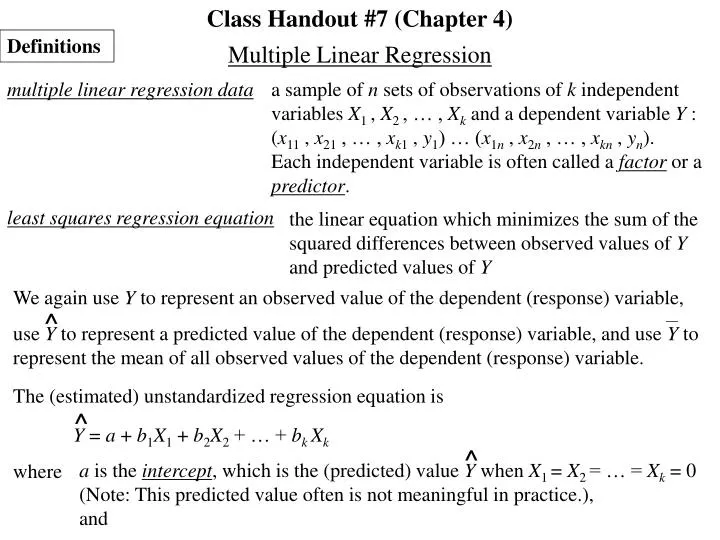
Class Handout #7 (Chapter 4). Definitions. Multiple Linear Regression. multiple linear regression data. a sample of n sets of observations of k independent variables X 1 , X 2 , … , X k and a dependent variable Y :

E N D
Class Handout #7 (Chapter 4) Definitions Multiple Linear Regression multiple linear regression data a sample of n sets of observations of k independent variables X1 , X2 , … , Xk and a dependent variable Y : (x11 , x21 , … , xk1 , y1) … (x1n , x2n , … , xkn , yn). Each independent variable is often called a factor or a predictor. least squares regression equation the linear equation which minimizes the sum of the squared differences between observed values of Y and predicted values of Y We again use Y to represent an observed value of the dependent (response) variable, use Y to represent a predicted value of the dependent (response) variable, and use Y to represent the mean of all observed values of the dependent (response) variable. ^ The (estimated) unstandardized regression equation is ^ Y = a + b1X1 + b2X2 + … + bk Xk ^ a is the intercept, which is the (predicted) value Y when X1 = X2 = … = Xk = 0 (Note: This predicted value often is not meaningful in practice.), and where
bi is the regression coefficient for Xi, which is the (estimated) amount Y changes on average with each increase of one unit in the variable Xi with all other independent variables (factors) remaining fixed. The (estimated) standardized linear equation is where ZY = 1ZX1 + 2ZX2 + … k ZXk i (beta) is the standardized regression coefficient for Xi , ZXi is the z-score for the value of Xi, and ZY is the z-score for the predicted value of Y. The ordinary (Pearson) correlation between two variables has been defined previously as a measure of strength of the linear relationship. A partial correlation is defined to be a measure of strength of the linear relationship between two variables given one more other variables. A standardized regression coefficient i is the partial correlation between Y and the corresponding Xi given all of the other Xis. As an example, consider how, among school children, the correlation between grip strength and height would be different from the partial correlation between grip strength and height given age.
Analysis of Variance (ANOVA) can be used to derive hypothesis tests in multiple regression, concerning the statistical significance of the overall regression and the statistical significance of individual independent variables (factors). The partitioning of the total sum of squares is analogous to that in simple linear regression. The basic ANOVA table can be organized as follows: k n – k – 1 n – 1 The f statistic in this ANOVA table is for deciding whether or not at least one regression coefficient is significantly different from zero (0), or in other words, whether or not the overall regression is statistically significant. Note that the regression degrees of freedom (df) is k (since the dependent variable is predicted from k independent variables), and that the total degrees of freedom is, as always, one less than the sample size n. Since the df for regression and the df for error must sum to the df for total, then the df for error must be equal to n – k – 1.
When one or more independent variables (factors) is added to a multiple regression model, then (1) the total sum of squares remains the same, (2) the regression sum of squares increases, (3) the error sum of squares decreases. A multiple regression model refers to a general equation which describes all of the independent variables from which the dependent variable Y is to be predicted. There are three types of independent variables that can be included in a multiple regression model: (1) (2) (3) a quantitative independent variable which is not a function of any other independent variable(s), or a higher-order term which refers to a function of one or more other independent variable(s), or a dummy (indicator) variable with possible values 0 or 1 each representing one of the categories of a dichotomy.
1. The data stored in the SPSS data file realestate is to be used in a study concerning the prediction of sale price of a residential property (dollars). Appraised land value (dollars), appraised value of improvements (dollars), and area of property living space (square feet) are to be considered as possible predictors, and the 20 properties selected for the data set are a random sample. Does the data appear to be observational or experimental? (a) Since the land value, improvement value, and area are all random, the data is observational. Use SPSS to do calculations necessary for multiple linear regression. Select the Analyze>Regression> Linear options, select the variable sale_prc for the Dependent slot, and select the variables land_val, impr_val, and area for the Independent(s) section. In the Method slot, select the Stepwise option. Click on the Statistics button, and make certain that the Estimates and Model fit options are selected in the dialog box which appears. Also, select the R squared change option, the Descriptives option, and the Collinearity diagnostics option. Click the Continue button to close the dialog box. Click on the Plots button, and select the Histogram option and the Normal Probability Plot option in the dialog box which appears. Also, from the list on the left, select ZRESID for the Y slot, and ZPRED for the X slot. Click the Continue button to close the dialog box. Finally, click the OK button. (b)
From the histogram of standardized residuals and the normal probability plot, comment on the normality assumption for a multiple regression. (c) Neither the histogram or the normal probability plot show evidence of serious departure from the normality assumption for a multiple regression. From the scatter plot of standardized predicted values and standardized residuals, comment on the linearity assumption and the homoscedasticity assumption for a multiple regression. (d) The scatter plot does not show any serious nonlinear pattern (i.e., no substantial departure from linearity), nor does it show any substantial difference in variation of the dependent variable as values of the independent variable(s) change (i.e., no substantial departure from homoscedasticity). From the Correlations table of the SPSS output comment on the possibility of multicollinearity in the multiple regression. (e) Since the correlation matrix does not contain any correlation greater than 0.8 for any pair of independent variables, it does not appear that multicollinearity will be a problem. Also, we see that tolerance > 0.10 (i.e., VIF < 10) for each independent variable.
From the Variables Entered/Removed table of the SPSS output, find the default values of the significance level to enter an independent variable into the model and the significance level to remove an independent variable from the model. (f) Respectively these are 0.05 and 0.10.
Regression Mean Square Total Mean Square The multiple R square is R2 = is the proportion (often converted to a percentage) of variation in the dependent variable Y accounted for by (or explained by) all of the independent variables X1 , X2 , … , Xk. The (positive) square root of R2 is sometimes called the multiple correlation coefficient. However, only the strength of the relationship between Y and more than one predictor can be considered; the direction of a relationship (positive or negative) can only be considered between Y and one predictor. When one or more independent variables (factors) is added to a multiple regression model, then since the total sum of squares remains the same and the regression sum of squares increases, then the value of R2 must increase. Since the value of R2 can be influenced by the sample size and the number of parameters in the model, an alternative measure of the strength of relationship between Y and all the predictors in a model is sometimes used. This alternative measure is called the adjusted R square denoted Ra2 and is defined by n – 1 Ra2 = 1 – ———— (1 –R2) . n – k– 1 It will always be true that 0 Ra2 R2 1 . The (estimated) standard error of estimate is s = Error Mean Square
When a large number of predictors are available in the prediction of a dependent variable Y, it is desirable to have some method for screening the predictors, that is, selecting those predictors which are most important. One possible method is to select independent variables that are significantly correlated with the dependent variable Y. A more sophisticated method is stepwise regression. Given that significance levels E and R are chosen respectively for entry and removal, stepwise regression is applied as follows: Note: The text description of stepwise regression is not quite correct. Step 1 All possible regressions with exactly one predictor are fit to the data. Among all predictors which are statistically significant at the Elevel, if any, the one for which the p-value is lowest (i.e., the one which is “most statistically significant”) is entered into the model, and Step 2 is performed next; if no predictors are statistically significant at the chosen Elevel, no predictors are entered into the model and the procedure ends. Step 2 Labeling the predictor entered into the model as X1, then all possible regressions with X1 and one other predictor are fit to the data. Among all predictors which are statistically significant with X1 in the model at the Elevel, if any, the one for which the p-value is lowest (i.e., the one which is “most statistically significant”) is entered into the model, and Step 3 is performed next; if no predictors are statistically significant with X1 in the model at the Elevel, no predictors are entered into the model and the procedure ends.
Step 3 Labeling the predictor entered into the model after X1 as X2, then a check is performed to see if X1 is statistically significant with X2 in the model at the Rlevel, and if not, then X1 is removed. Next, Step 4 is performed. Step 4 All possible regressions with the predictor(s) currently in the model and one other predictor are fit to the data. Among all predictors which are statistically significant after the predictor(s) currently in the model at the E level, if any, the one for which p-value is lowest (i.e., the one which is “most statistically significant”) is entered into the model, and Step 5 is performed next; if no predictors are statistically significant after the predictor(s) currently in the model at the Elevel, no predictors are entered into the model and the procedure ends. Step 5 A check is then performed to see if each of the predictors in the model is statistically significant with all other predictors now in the model. Among all predictors which are not statistically significant at the Rlevel, if any, the one for which the p-value is highest is removed from the model, and the check is repeated until no more variables can be removed. Step 6 Steps 4 and 5 are repeated successively until no more variables can be entered or removed .
Other methods to decide which of many predictors are the most important include the forward selection method (which is the same as stepwise regression except there is no option to remove variables from the model), the backward elimination method (where we begin with all predictors in the model and remove the most statistically insignificant at each step until no more predictors can be removed), and various methods which depend on doing all possible regressions (discussed in Section 6.3). The hypothesis test to decide whether or not a predictor is statistically significant when entered into a model after other predictors are already in the model is equivalent to the hypothesis test to decide whether or not the partial correlation between the dependent variable Y and the predictor being entered into the model given all the predictors already in the model is statistically significant. The results of only one method with one data set to select the most important predictors should not be considered final. Typically, further analysis is necessary. For instance, several procedures could be used with the same data to see if the same results are obtained. Higher order terms can also be investigated.
Multicollinearity is said to be present among a set of independent variables when there is at least one high correlation among two of the independent variables or among two different linear combinations of the independent variables. Multicollinearity can cause problems with the calculations involved in a multiple linear regression. Often, multicollinearity can be detected by observing that the correlation between a pair of independent variables is larger than 0.80. The tolerance for any given independent variable is the proportion of variance in that independent variable unexplained by the other independent variables, and the variance inflation factor (VIF) is the reciprocal of the tolerance. A multicollinearity problem is indicated by tolerance < 0.10, that is, VIF > 10. Pages 101 to 103 of the textbook list the assumptions on which the ANOVA for a multiple linear regression is based. These assumptions include a normal distribution for the dependent variable at any given combination of values for the independent variables in the multiple linear regression , and also include a linear relationship with each independent variable and a homoscedasticity assumption (equal variance of the dependent variable no matter what the values of the independent varaible(s)). If these assumptions are satisfied, then the ANOVA for a multiple linear regression is an appropriate statistical technique.
1.-continued From the Variables Entered/Removed table of the SPSS output, find the (g) number of steps in the stepwise multiple regression, and list the independent variables selected and removed at each step. There were two steps in the stepwise multiple regression; the variable “appraised value of improvements” was entered in the first step, and the variable “area of property living space” was entered in the second step. No variables were removed at either step. From the Correlations table of the SPSS output, find the ordinary correlation between the dependent variable sale price and the first independent variable entered into the model. (h) The correlation between sale price and appraised value of improvements is 0.916.
From the Coefficients table of the SPSS output, find the partial correlation between the dependent variable sale price and the second independent variable entered into the model given the first independent variable entered into the (i) model; compare this to the ordinary correlation between the dependent variable sale price and the second independent variable entered into the model, which can be found from the Correlations table of the SPSS output. The partial correlation between sale price and area of property living space given appraised value of improvements is 0.515. The ordinary correlation between sale price and area of property living space is 0.849.
From the Model Summary table of the SPSS output, find the change(s) in R2 from the model at one step to the next step. (j) From the model at Step 1, we see that “appraised value of improvements” accounts for 83.8% of the variance in “sale price”. From the model at Step 2, we see that “appraised value of improvements” and “area of property living space” together account for 88.1% of the variance in “sale price”. With “appraised value of improvements” already in the model, “area of property living space” accounts for an additional 4.3% of the variance in “sale price”.
1.-continued From the Coefficients table of the SPSS output, write the estimated regression equation for each step. (k) sale_prc = 8945.575 + 1.351(impr_val) Step 1: Step 2: sale_prc = 97.521 + 0.960(impr_val) + 16.373(area)
Use the estimated regression equation from the final step of the stepwise multiple regression to predict the sale price of a residential property where the appraised land value is $8000, the appraised value of improvements is $20,000, and area of property living space is 1200 square feet. (l) 97.521 + 0.960(20000) + 16.373(1200) = $38,945.12
A dummy (indicator) variable is one defined to be 1 if a given condition is satisfied and 0 otherwise. Suppose a qualitative-dichotomous variable is to be used in a regression model to predict a dependent variable Y. If we label the categories (levels) of the qualitative-dichotomous variable as #1 and #2, then this variable can be represented by defining an appropriate dummy variable, such as 1 for category #1 X = 0 for category #2 A regression equation to predict Y from X can be written as Y = a + bX . ^ ^ a + b(0) = a . When X = 0, then the predicted value for Y is Y = ^ a + b(1) = When X = 1, then the predicted value for Y is Y = a + b . b = amount that predicted Y for category #1 exceeds predicted Y for category #2.
Suppose a qualitative variable with 3 categories (levels) is to be used in a regression model to predict a dependent variable Y. If we label the categories as #1, #2, and #3, then this qualitative variable can be represented by defining two appropriate dummy variables, such as 1 for category #1 X1 = 0 otherwise 1 for category #2 X2 = 0 otherwise and A regression equation to predict Y from X1 and X2 can be written as Y = a + b1X1 + b2X2 . ^ ^ a + b1(0) + b2(0) = a . When X1 = 0 and X2 = 0, then the predicted value for Y is Y = ^ a + b1(1) + b2(0) = When X1 = 1 and X2 = 0, then the predicted value for Y is Y = a + b1 . ^ a + b1(0) + b2(1) = When X1 = 0 and X2 = 1, then the predicted value for Y is Y = a + b2 . b1 = amount that predicted Y for category #1 exceeds predicted Y for category #3. b2 = amount that predicted Y for category #2 exceeds predicted Y for category #3. In practice, which categories are associated with which dummy variables does not matter. The category which is not associated with any dummy variable is sometimes called the reference group (since each coefficient in the regression model represents a difference in mean when this group is compared to one other group).
Suppose a qualitative variable with k categories (levels) is to be used in a regression model to predict a dependent variable Y. If we label the categories as #1, #2, …, #k, then this qualitative variable can be represented by defining k– 1 appropriate dummy variables, such as 1 for category #1 X1 = 0 otherwise 1 for category # k– 1 Xk– 1 = 0 otherwise . . . A regression equation to predict Y from X1 , X2 , … , Xk 1 can be written as Y = a + b1X1 + b2X2 + … + bk 1 Xk 1 . ^ ^ a + b1(0) + b2(0) = a . When X1 = 0 and X2 = 0, then the predicted value for Y is Y = ^ a + b1(1) + b2(0) = When X1 = 1 and X2 = 0, then the predicted value for Y is Y = a + b1 . ^ a + b1(0) + b2(1) = When X1 = 0 and X2 = 1, then the predicted value for Y is Y = a + b2 . bi = amount that predicted Y for category #i exceeds predicted Y for category # k. When a qualitative variable has k categories (levels) with k > 2, the k– 1 dummy variables X1 , X2 , … , Xk– 1 are treated as a group so that either all of them are included in the model or none of them are included in the model. An alternative approach (used in the textbook) is to define one more dummy variable Xk corresponding to category #k, and treating the k dummy variables as separate, individual variables.
2. A company conducts a study to see how diastolic blood pressure is influenced by an employee’s age, weight, and job stress level classified as high stress, some stress, and low stress. A 0.05 significance level is chosen for an analysis of covariance. Data recorded on 24 employees treated as a random sample is displayed on the right. The data has been stored in the SPSS data file jobstress. Diastolic Job Age Weight Blood Stress (years) (lbs.) Pressure High 23 208 102 High 43 215 126 High 34 175 110 High 65 162 124 High 39 197 120 High 35 160 113 High 29 100 81 High 25 188 100 Some 38 164 97 Some 19 173 93 Some 24 209 92 Some 32 150 93 Some 47 209 120 Some 54 212 115 Some 57 112 93 Some 43 215 116 Low 61 162 103 Low 27 116 81 By following the instructions below, add the following dummy variables for job stress level to the SPSS data file jobstress: (a) 1 for high stress job X1 = 0 otherwise 1 for some stress job X2 = 0 otherwise 1 for low stress job X3 = 0 otherwise
Select the Transform> Recode into Different Variablesoptions in SPSS. In the dialog box which appears, select the variable jobtype for the Numeric Variable -> Output Variable section. In the Output Variable section, type X1 in the Name slot of the Output Variable section. Low 40 142 83 Low 26 116 81 Low 36 160 93 Low 50 212 109 Low 59 201 116 Low 49 217 110 Click the Change button to make X1 the output variable, which is indicated in the Numeric Variable -> Output Variable section. Click the Old and New Values button. In the dialog box which appears, type 3 in the Value slot of the Old Value section, type 1 in the Value slot of the New Value section, and click the Add button. You should now see an indication that the value 3 for the variable jobtype will correspond to a value of 1 for the variable X1. In a similar manner, set the value 2 for the variable jobtype to correspond to a value of 0 for the variable X1, and set the value 1 for the variable jobtype to correspond to a value of 0 for the variable X1. Click the Continue button to close the dialog box. Finally, click the OK button, after which you should see that variable X1 has been added to the data, and that its values are correct. Now, using a procedure similar to that for defining variable X1, define variables X2 and X3.
2.-continued Use the Analyze> Regression> Linear> options in SPSS to display the Linear Regression dialog box. Select the variable dbp for the Dependent slot, select the variables age, weight, X1, X2, and X3, for the Independent(s) section. In the Method slot, select the Stepwise option. Click on the Statistics button, and make certain that the Estimates and Model fit options are selected in the dialog box which appears. Also, select the R squared change option, the Descriptives option, and the Collinearity diagnostics option. Click the Continue button to close the dialog box. Click on the Plots button, and select the Histogram option and the Normal Probability Plot option in the dialog box which appears. Also, from the list on the left, select ZRESID for the Y slot, and ZPRED for the X slot. Click the Continue button to close the dialog box. Finally, click the OK button. (b) From the histogram of standardized residuals and the normal probability plot, comment on the normality assumption for a multiple regression. (c) Neither the histogram or the normal probability plot show evidence of serious departure from the normality assumption for a multiple regression.
From the scatter plot of standardized predicted values and standardized residuals, comment on the linearity assumption and the homoscedasticity assumption for a multiple regression. (d) The scatter plot does not show any serious nonlinear pattern (i.e., no substantial departure from linearity), nor does it show any substantial difference in variation of the dependent variable as values of the independent variable(s) change (i.e., no substantial departure from homoscedasticity). From the Correlations table of the SPSS output comment on the possibility of multicollinearity in the multiple regression. (e) Since the correlation matrix does not contain any correlation greater than 0.8 for any pair of independent variables, it does not appear that multicollinearity will be a problem. Also, we see that tolerance > 0.10 (i.e., VIF < 10) for each independent variable From the Variables Entered/Removed table of the SPSS output, find the default values of the significance level to enter an independent variable into the model and the significance level to remove an independent variable from the model. (f) Respectively these are 0.05 and 0.10.
2.-continued From the Variables Entered/Removed table of the SPSS output, find the number of steps in the stepwise multiple regression, and list the independent variables selected and removed at each step. (g) There were three steps in the stepwise multiple regression; the variable weight was entered in the first step, the variable age was entered in the second step, and the variable X1 was entered in the third step. No variables were removed at any step.
From the Correlations table of the SPSS output, find the ordinary correlation between the dependent variable diastolic blood pressure and the first independent variable entered into the model. (h) The correlation between diastolic blood pressure and weight is 0.727.
From the Coefficients table of the SPSS output, find the partial correlation between the dependent variable diastolic blood pressure and the second independent variable entered into the model given the first independent variable entered into the model; compare this to the ordinary correlation between the dependent variable diastolic blood pressure and the second independent variable entered into the model, which can be found from the Correlations table of the SPSS output. (i) The partial correlation between diastolic blood pressure and age given weight is 0.442. The ordinary correlation between diastolic blood pressure and age is 0.561.
From the Model Summary table of the SPSS output, find the change(s) in R2 from the model at one step to the next step. (j) From the model at Step 1, we see that weight accounts for 52.8% of the variance in diastolic blood pressure. From the model at Step 2, we see that weight and age together account for 71.8% of the variance in diastolic blood pressure. With weight already in the model, age accounts for an additional 19.0% of the variance in diastolic blood pressure. From the model at Step 3, we see that weight, age, and the variable X1 together account for 87.3% of the variance in diastolic blood pressure. With weight and age already in the model, the variable X1 accounts for an additional 15.5% of the variance in diastolic blood pressure.
2.-continued From the Coefficients table of the SPSS output, write the estimated regression equation for each step. (k) dbp = 54.266 + 0.280(weight) Step 1: Step 2: Step 3: dbp = 40.653 + 0.249(weight) + 0.478(age) dbp = 35.279 + 0.238(weight) + 0.559(age) + 11.871(X1) Use the estimated regression equation from the final step of the stepwise multiple regression to predict the diastolic blood pressure of an employee whose weight is 180 lbs, whose age is 35, and whose job stress level is classified to be “high”. (l) dbp = 35.279 + 0.238(180) + 0.559(35) + 11.871(1) = 109.555
Use the estimated regression equation from the final step of the stepwise multiple regression to predict the diastolic blood pressure of an employee whose weight is 180 lbs, whose age is 35, and whose job stress level is classified to be “some”. (m) dbp = 35.279 + 0.238(180) + 0.559(35) + 11.871(0) = 97.684 Use the estimated regression equation from the final step of the stepwise multiple regression to predict the diastolic blood pressure of an employee whose weight is 180 lbs, whose age is 35, and whose job stress level is classified to be “low”. (n) dbp = 35.279 + 0.238(180) + 0.559(35) + 11.871(0) = 97.684
3. Read the “INTRODUCTION” and “MULTIPLE LINEAR REGRESSION ANALYSIS” sections of Chapter 4. Open the version of the SPSS data file Job Satisfaction that was saved after Exercise #10 on Class Handout #5. (a) In the “PRACTICAL EXAMPLE” section, read the discussion for assumptions number 1 to 6 in the subsection “Hypothesis Testing”; then, use the Analyze> Descriptive Statistics> Explore options in SPSS to obtain Figure 4.1 and Table 4.1, and use the Graphs> Legacy Dialogs> Scatter/Dot options in SPSS to obtain Figure 4.2. (The other tables and figures displayed in this subsection can be obtained from work to be done in the subsection which follows.) (b) In the “PRACTICAL EXAMPLE” section, read the discussion for assumptions number 7 and 8 in the subsection “Hypothesis Testing” and the remaining portion of the subsection; then, use the Transform> Recode into Different Variables options in SPSS to create the dummy variables discussed with regard to assumption number 7. Compare the syntax file commands generated by the output with those shown on page 110 of the textbook.
(c) In the “PRACTICAL EXAMPLE” section, read the subsection “How to Use SPSS to Compute Multiple Regression Coefficients”, and follow the instructions with SPSS, which should produce much of the output displayed in Table 4.2 to Table 4.12 and in Figures 4.3 and 4.4. Compare the syntax file commands generated by the output with those shown on page 116 of the textbook. Read the remaining portion of Chapter 4.