Download
1 / 50
500 likes | 674 Views
MGMT 276: Statistical Inference in Management Spring, 2014. Welcome. Green sheets. Please hand in your homework. Please click in. My last name starts with a letter somewhere between A. A – D B. E – L C. M – R D. S – Z . For our class Due Tuesday April 29 th. For our class

E N D
MGMT 276: Statistical Inference in ManagementSpring, 2014 Welcome Green sheets
Please hand in your homework Please click in My last name starts with a letter somewhere between A. A – D B. E – L C. M – R D. S – Z
For our class Due Tuesday April 29th
For our class Due Tuesday April 29th
Readings for next exam (Exam 4: May 1st) Lind Chapter 13: Linear Regression and Correlation Chapter 14: Multiple Regression Chapter 15: Chi-Square Plous Chapter 17: Social Influences Chapter 18: Group Judgments and Decisions
Exam 4 – Optional Times for Final • Two options for completing Exam 4 • Thursday (5/1/14) – The regularly scheduled time • Tuesday (5/6/14) – The optional later time • Must sign up to take Exam 4 on Tuesday (4/29) • Only need to take one exam – these are two optional times
Homework due – Tuesday (April 29th) • On class website: • Please print and complete homework worksheet #19 & 20 • Using Excel for Multiple Regression
Use this as your study guide Next couple of lectures 4/24/14 Logic of hypothesis testing with Correlations Interpreting the Correlations and scatterplots Simple and Multiple Regression Using correlation for predictions r versus r2 Regression uses the predictor variable (independent) to make predictions about the predicted variable (dependent)Coefficient of correlation is name for “r”Coefficient of determination is name for “r2”(remember it is always positive – no direction info)Standard error of the estimate is our measure of the variability of the dots around the regression line(average deviation of each data point from the regression line – like standard deviation) Coefficient of regression will “b” for each variable (like slope)
Correlation: Independent and dependent variables • When used for prediction we refer to the predicted variable • as the dependent variable and the predictor variable as the independent variable What are we predicting? What are we predicting? Dependent Variable Dependent Variable Independent Variable Independent Variable
Multiple regression equations 1 How many independent variables? How many dependent variables? Prediction line Y’ = b1X 1+ b0 • We can predict amount of crime in a city from • the number of bathrooms in city Prediction line Y’ = b1X 1+ b2X 2+ b0 • We can predict amount of crime in a city from • the number of bathrooms in city • the amount spent on education in city 3 How many independent variables? 1 How many dependent variables? Prediction line Y’ = b1X 1+ b2X 2+ b3X 3+ b0 • We can predict amount of crime in a city from • the number of bathrooms in city • the amount spent on education in city • the amount spent on after-school programs
Multiple regression • Used to describe the relationship between several independent variables and a dependent variable. Can we predict amount of crime in a city from the number of bathrooms and the amount of spent on education and on after-school programs? Prediction line Y’ = b1X 1+ b2X 2+ b3X 3+ b0 • X1 X2 and X3are the independent variables. • Y is the dependent variable (amount of crime) • b0is the Y-intercept • b1is the net change in Y for each unit change in X1 holding X2and X3 constant. It is called a regressioncoefficient.
YearlyIncome Expenses per year Multiple regression will use multiple independent variables to predict the single dependent variable You probably make this much The predicted variable goes on the “Y” axis and is called the dependent variable. The predictor variable goes on the “X” axis and is called the independent variable You probably make this much Dependent Variable (Predicted) If you spend this much If you save this much Independent Variable 1 (Predictor) If you spend this much Independent Variable 2 (Predictor)
Regression Plane for a 2-Independent Variable Linear Regression Equation
Multiple regression equations • Can use variables to predict • behavior of stock market • probability of accident • amount of pollution in a particular well • quality of a wine for a particular year • which candidates will make best workers
Can use variables to predict which candidates will make best workers • Measured current workers – the best workers tend to have highest “success scores”. (Success scores range from 1 – 1,000) • Try to predict which applicants will have the highest success score. • We have found that these variables predict success: • Age (X1) • Niceness (X2) • Harshness (X3) Both 10 point scales Niceness (10 = really nice) Harshness (10 = really harsh) According to your research, age has only a small effect on success, while workers’ attitude has a big effect. Turns out, the best workers have high “niceness” scores and low “harshness” scores. Your results are summarized by this regression formula: Y’ = b1X 1+ b2X 2+ b3X 3 + a Y’ = b1 X1 + b2 X2 + b3 X 3 + a Success score = (1)(Age) + (20)(Nice) + (-75)(Harsh) + 700
According to your research, age has only a small effect on success, while workers’ attitude has a big effect. Turns out, the best workers have high “niceness” scores and low “harshness” scores. Your results are summarized by this regression formula: Y’ = b1 X1 + b2 X2 + b3 X 3 + a Success score = (1)(Age) + (20)(Nice) + (-75)(Harsh) + 700
According to your research, age has only a small effect on success, while workers’ attitude has a big effect. Turns out, the best workers have high “niceness” scores and low “harshness” scores. Your results are summarized by this regression formula: Y’ = b1 X1 + b2 X2 + b3 X 3 + a Success score = (1)(Age) + (20)(Nice) + (-75)(Harsh) + 700 • Y’ is the dependent variable • “Success score” is your dependent variable. • X1 X2 and X3are the independent variables • “Age”, “Niceness” and “Harshness” are the independent variables. • Each “b” is called a regression coefficient. • Each “b” shows the change in Y for each unit change in its own X (holding the other independent variables constant). • a is the Y-intercept
Y’ = b1X 1 + b2X 2 + b3X 3+ a The Multiple Regression Equation – Interpreting the Regression Coefficients Success score = (1)(Age) + (20)(Nice) + (-75)(Harsh) + 700 b1 = The regression coefficient for age (X1) is “1” The coefficient is positive and suggests a positive correlation between age and success. As the age increases the success score increases. The numeric value of the regression coefficient provides more information. If age increases by 1 year and hold the other two independent variables constant, we can predict a 1 point increase in the success score.
Y’ = b1X 1 + b2X 2 + b3X 3+ a The Multiple Regression Equation – Interpreting the Regression Coefficients Success score = (1)(Age) + (20)(Nice) + (-75)(Harsh) + 700 b2 = The regression coefficient for age (X2) is “20” The coefficient is positive and suggests a positive correlation between niceness and success. As the niceness increases the success score increases. The numeric value of the regression coefficient provides more information. If the “niceness score” increases by one, and hold the other two independent variables constant, we can predict a 20 point increase in the success score.
Y’ = b1X 1 + b2X 2 + b3X 3+ a The Multiple Regression Equation – Interpreting the Regression Coefficients Success score = (1)(Age) + (20)(Nice) + (-75)(Harsh) + 700 b3 = The regression coefficient for age (X3) is “-75” The coefficient is negative and suggests a negative correlation between harshness and success. As the harshness increases the success score decreases. The numeric value of the regression coefficient provides more information. If the “harshness score” increases by one, and hold the other two independent variables constant, we can predict a 75 point decrease in the success score.
Here comes Victoria, her scores are as follows: Prediction line: Y’ = b1X 1+ b2X 2+ b3X 3+ a Y’ = 1X 1+ 20X 2- 75X 3+ 700 Y' = (1)(Age) + (20)(Nice) + (-75)(Harsh) + 700 • Age = 30 • Niceness = 8 • Harshness= 2 Y' = (1)(Age) + (20)(Nice) + (-75)(Harsh) + 700 What would we predict her “success index” to be? Y' = (1)(Age) + (20)(Nice) + (-75)(Harsh) + 700 We predict Victoria will have a Success Index of 740 (1)(30) - 75(2) + (20)(8) + 700 Y’ = = 3.812 Y’ = 740 Y' = (1)(Age) + (20)(Nice) + (-75)(Harsh) + 700
Here comes Victoria, her scores are as follows: Prediction line: Y’ = b1X 1+ b2X 2+ b3X 3+ a Y’ = 1X 1+ 20X 2- 75X 3+ 700 Y' = (1)(Age) + (20)(Nice) + (-75)(Harsh) + 700 • Age = 30 • Niceness = 8 • Harshness= 2 Y' = (1)(Age) + (20)(Nice) + (-75)(Harsh) + 700 What would we predict her “success index” to be? Y' = (1)(Age) + (20)(Nice) + (-75)(Harsh) + 700 We predict Victoria will have a Success Index of 740 (1)(30) - 75(2) Y’ = + (20)(8) + 700 = 3.812 Y’ = 740 Here comes Victor, his scores are as follows: We predict Victor will have a Success Index of 175 • Age = 35 • Niceness = 2 • Harshness= 8 What would we predict his “success index” to be? Y' = (1)(Age) + (20)(Nice) + (-75)(Harsh) + 700 (1)(35) - 75(8) + (20)(2) + 700 Y’ = Y’ = 175
Can use variables to predict which candidates will make best workers We predict Victor will have a Success Index of 175 We predict Victoria will have a Success Index of 740 Who will we hire?
Multiple Linear Regression - Example Can we predict heating cost? Three variables are thought to relate to the heating costs: (1) the mean daily outside temperature, (2) the number of inches of insulation in the attic, and (3) the age in years of the furnace. To investigate, Salisbury's research department selected a random sample of 20 recently sold homes. It determined the cost to heat each home last January
The Multiple Regression Equation – Interpreting the Regression Coefficients b1 = The regression coefficient for mean outside temperature (X1) is -4.583. The coefficient is negative and shows a negative correlation between heating cost and temperature. As the outside temperature increases, the cost to heat the home decreases. The numeric value of the regression coefficient provides more information. If we increase temperature by 1 degree and hold the other two independent variables constant, we can estimate a decrease of $4.583 in monthly heating cost.
The Multiple Regression Equation – Interpreting the Regression Coefficients b2 = The regression coefficient for mean attic insulation (X2) is -14.831. The coefficient is negative and shows a negative correlation between heating cost and insulation. The more insulation in the attic, the less the cost to heat the home. So the negative sign for this coefficient is logical. For each additional inch of insulation, we expect the cost to heat the home to decline $14.83 per month, regardless of the outside temperature or the age of the furnace.
The Multiple Regression Equation – Interpreting the Regression Coefficients b3 = The regression coefficient for mean attic insulation (X3) is 6.101 The coefficient is positive and shows a negative correlation between heating cost and insulation. As the age of the furnace goes up, the cost to heat the home increases. Specifically, for each additional year older the furnace is, we expect the cost to increase $6.10 per month.
Applying the Model for Estimation What is the estimated heating cost for a home if: • the mean outside temperature is 30 degrees, • there are 5 inches of insulation in the attic, and • the furnace is 10 years old?
Multiple regression equations Very often we want to select students or employees who have the highest probability of success in our school or company. Andy is an administrator at a paralegal program and he wants to predict the Grade Point Average (GPA) for the incoming class. He thinks these independent variables will be helpful in predicting GPA. • High School GPA (X1) • SAT - Verbal (X2) • SAT - Mathematical (X3) Andy completes a multiple regression analysis and comes up with this regression equation: Prediction line Y’ = b1X 1+ b2X 2+ b3X 3+ a Y’ = 1.2X 1+ .00163X 2- .00194X 3 - .411 Y’ = 1.2 gpa + .00163satverb - .00194satmath - .411
Here comes Victoria, her scores are as follows: Prediction line: Y’ = b1X 1+ b2X 2+ b3X 3+ a Y’ = 1.2X 1+ .00163X 2-.00194X 3 - .411 • High School GPA = 3.81 • SATVerbal = 500 • SATMathematical = 600 What would we predict her GPA to be in the paralegal program? Y’ = 1.2 gpa + .00163satverb - .00194satmath - .411 Y’ = 1.2 (3.81)+ .00163(500)- .00194 (600)- .411 We predict Victoria will have a GPA of 3.812 Y’ = 4.572 + .815 - 1.164 - .411 = 3.812 Predict Victor’s GPA, his scores are as follows: We predict Victor will have a GPA of 2.656 • High School GPA = 2.63 • SAT - Verbal = 469 • SAT - Mathematical = 440 Y’ = 1.2 gpa + .00163satverb - .00194 satmath - .411 Y’ = 1.2 (2.63)+ .00163(469)- .00194 (440)- .411 = 2.66 Y’ = 3.156 + .76447 - .8536 - .411
What if we were looking to see if our stop-smoking program affects peoples‘ desire to smoke. What would null hypothesis be? a. Can’t know without knowing the dependent variable b. The program does not work c. The programs works d. Comparing the null and alternative hypothesis Correct
Correct Which of the following is a Type I error: a. We conclude that the program works when it fact it doesn’t b. We conclude that the program works when in fact it does c. We conclude that the program doesn’t work when in fact it does d. We conclude that the program doesn’t work when in fact it doesn’t
What is the null hypothesis of a correlation coefficient? a. It is zero (nothing going on)b. It is less than zeroc. It is more than zerod. It equals the computed sample correlation Correct
Let’s try one Winnie found an observed correlation coefficient of 0, what should she conclude? a. Reject the null hypothesis b. Do not reject the null hypothesis c. Not enough info is given Correct
In the regression equation, what does the letter "a" represent? a. Y interceptb. Slope of the linec. Any value of the independent variable that is selectedd. None of these Correct Y’ = a + bx1+ bx2 + bx3 + bx4
Assume the least squares equation is Y’ = 10 + 20X. What does the value of 10 in the equation indicate? a. Y interceptb. For each unit increased in Y, X increases by 10c. For each unit increased in X, Y increases by 10d. None of these . Correct
In the least squares equation, Y’ = 10 + 20X the value of 20 indicates a. the Y intercept.b for each unit increase in X, Y increases by 20.c. for each unit increase in Y, X increases by 20.d. none of these. Correct
In the equation Y’ = a + bX, what is Y’ ? a. Slope of the lineb. Y interceptC. Predicted value of Y, given a specific X valued. Value of Y when X = 0 Correct
If there are four independent variables in a multiple regression equation, there are also four a. Y-intercepts (a).b. regression coefficients (slopes or bs).c. dependent variables.d. constant terms (k). Correct Y’ = a + bx1+ bx2 + bx3 + bx4
According to the Central Limit Theorem, which is false? As n ↑ xwill approach µ a. b. As n ↑ curve will approach normal shape As n ↑ curve variability gets larger c. Correct As n ↑ d.
If the coefficient of determination (r2) is 0.80, what percent of variation is explained? a. 20%b. 90%c. 64%d. 80% Correct What percent of variation is not explained? a. 20%b. 90%c. 64%d. 80% Correct
Which of the following represents a significant finding: a. p < 0.05 b. t(3) = 0.23; n.s. c. the observed t statistic is nearly zero d. we do not reject the null hypothesis Correct
Thank you! See you next time!!