Download
1 / 49
530 likes | 868 Views
Hierarchical Clustering. Adapted from Slides by Prabhakar Raghavan, Christopher Manning, Ray Mooney and Soumen Chakrabarti. “The Curse of Dimensionality”. Why document clustering is difficult

E N D
Hierarchical Clustering Adapted from Slides by Prabhakar Raghavan, Christopher Manning, Ray Mooney and Soumen Chakrabarti L14HierCluster
“The Curse of Dimensionality” • Why document clustering is difficult • While clustering looks intuitive in 2 dimensions, many of our applications involve 10,000 or more dimensions… • High-dimensional spaces look different • The probability of random points being close drops quickly as the dimensionality grows. • Furthermore, random pair of vectors are all almost perpendicular.
Today’s Topics • Hierarchical clustering • Agglomerative clustering techniques • Evaluation • Term vs. document space clustering • Multi-lingual docs • Feature selection • Labeling
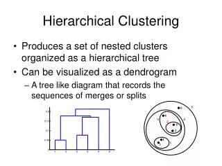
animal vertebrate invertebrate fish reptile amphib. mammal worm insect crustacean Hierarchical Clustering • Build a tree-based hierarchical taxonomy (dendrogram) from a set of documents. • One approach: recursive application of a partitional clustering algorithm.
Dendogram: Hierarchical Clustering • Clustering obtained by cutting the dendrogram at a desired level: each connected component forms a cluster.
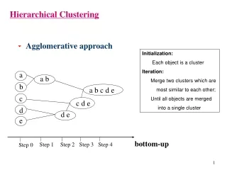
Hierarchical Clustering algorithms • Agglomerative (bottom-up): • Start with each document being a single cluster. • Eventually all documents belong to the same cluster. • Divisive (top-down): • Start with all documents belong to the same cluster. • Eventually each node forms a cluster on its own. • Does not require the number of clusters k in advance • Needs a termination/readout condition • The final mode in both Agglomerative and Divisive is of no use.
Hierarchical Agglomerative Clustering (HAC) Algorithm Start with all instances in their own cluster. Until there is only one cluster: Among the current clusters, determine the two clusters, ci and cj, that are most similar. Replace ci and cj with a single cluster ci cj
d3,d4,d5 d4,d5 d3 Dendrogram: Document Example • As clusters agglomerate, docs likely to fall into a hierarchy of “topics” or concepts. d3 d5 d1 d4 d2 d1,d2
Key notion: cluster representative • We want a notion of a representative point in a cluster, to represent the location of each cluster • Representative should be some sort of “typical” or central point in the cluster, e.g., • point inducing smallest radii to docs in cluster • smallest squared distances, etc. • point that is the “average” of all docs in the cluster • Centroid or center of gravity • Measure intercluster distances by distances of centroids.
Centroid after second step. Centroid after first step. Example: n=6, k=3, closest pair of centroids d4 d6 d3 d5 d1 d2
Centroid Outliers in centroid computation • Can ignore outliers when computing centroid. • What is an outlier? • Lots of statistical definitions, e.g. • moment of point to centroid > M some cluster moment. Say 10. Outlier
Closest pair of clusters • Many variants to defining closest pair of clusters • Single-link • Similarity of the most cosine-similar (single-link) • Complete-link • Similarity of the “furthest” points, the least cosine-similar • Centroid • Clusters whose centroids (centers of gravity) are the most cosine-similar • Average-link • Average cosine between pairs of elements
Single Link Agglomerative Clustering • Use maximum similarity of pairs: • Can result in “straggly” (long and thin) clusters due to chaining effect. • After merging ci and cj, the similarity of the resulting cluster to another cluster, ck, is:
Complete Link Agglomerative Clustering • Use minimum similarity of pairs: • Makes “tighter,” spherical clusters that are typically preferable. • After merging ci and cj, the similarity of the resulting cluster to another cluster, ck, is: Ci Cj Ck
Computational Complexity • In the first iteration, all HAC methods need to compute similarity of all pairs of n individual instances which is O(n2). • In each of the subsequent n2 merging iterations, compute the distance between the most recently created cluster and all other existing clusters. • In order to maintain an overall O(n2) performance, computing similarity to each cluster must be done in constant time. • Else O(n2log n) or O(n3) if done naively
Group Average Agglomerative Clustering • Use average similarity across all pairs within the merged cluster to measure the similarity of two clusters. • Compromise between single and complete link. • Two options: • Averaged across all ordered pairs in the merged cluster • Averaged over all pairs between the two original clusters • Some previous work has used one of these options; some the other. No clear difference in efficacy
Computing Group Average Similarity • Assume cosine similarity and normalized vectors with unit length. • Always maintain sum of vectors in each cluster. • Compute similarity of clusters in constant time:
Efficiency: Medoid As Cluster Representative • The centroid does not have to be a document. • Medoid: A cluster representative that is one of the documents • For example: the document closest to the centroid • One reason this is useful • Consider the representative of a large cluster (>1000 documents) • The centroid of this cluster will be a dense vector • The medoid of this cluster will be a sparse vector • Compare: mean/centroid vs. median/medoid
Efficiency: “Using approximations” • In standard algorithm, must find closest pair of centroids at each step • Approximation: instead, find nearly closest pair • use some data structure that makes this approximation easier to maintain • simplistic example: maintain closest pair based on distances in projection on a random line Random line
Term vs. document space • So far, we clustered docs based on their similarities in term space • For some applications, e.g., topic analysis for inducing navigation structures, can “dualize” • use docs as axes • represent (some) terms as vectors • proximity based on co-occurrence of terms in docs • now clustering terms, not docs
Term vs. document space • Cosine computation • Constant for docs in term space • Grows linearly with corpus size for terms in doc space • Cluster labeling • Clusters have clean descriptions in terms of noun phrase co-occurrence • Application of term clusters
Multi-lingual docs • E.g., Canadian government docs. • Every doc in English and equivalent French. • Must cluster by concepts rather than language • Simplest: pad docs in one language with dictionary equivalents in the other • thus each doc has a representation in both languages • Axes are terms in both languages
Feature selection • Which terms to use as axes for vector space? • Large body of (ongoing) research • IDF is a form of feature selection • Can exaggerate noise e.g., mis-spellings • Better to use highest weight mid-frequency words – the most discriminating terms • Pseudo-linguistic heuristics, e.g., • drop stop-words • stemming/lemmatization • use only nouns/noun phrases • Good clustering should “figure out” some of these
Major issue - labeling • After clustering algorithm finds clusters - how can they be useful to the end user? • Need pithy label for each cluster • In search results, say “Animal” or “Car” in the jaguar example. • In topic trees (Yahoo), need navigational cues. • Often done by hand, a posteriori.
How to Label Clusters • Show titles of typical documents • Titles are easy to scan • Authors create them for quick scanning! • But you can only show a few titles which may not fully represent cluster • Show words/phrases prominent in cluster • More likely to fully represent cluster • Use distinguishing words/phrases • Differential labeling
Labeling • Common heuristics - list 5-10 most frequent terms in the centroid vector. • Drop stop-words; stem. • Differential labeling by frequent terms • Within a collection “Computers”, clusters all have the word computer as frequent term. • Discriminant analysis of centroids. • Perhaps better: distinctive noun phrase
What is a Good Clustering? • Internal criterion: A good clustering will produce high quality clusters in which: • the intra-class (that is, intra-cluster) similarity is high • the inter-class similarity is low • The measured quality of a clustering depends on both the document representation and the similarity measure used
External criteria for clustering quality • Quality measured by its ability to discover some or all of the hidden patterns or latent classes in gold standard data • Assesses a clustering with respect to ground truth • Assume documents with C gold standard classes, while our clustering algorithms produce K clusters, ω1, ω2, …, ωK with nimembers.
External Evaluation of Cluster Quality • Simple measure: purity, the ratio between the dominant class in the cluster πi and the size of cluster ωi • Others are entropy of classes in clusters (or mutual information between classes and clusters)
Purity example Cluster I Cluster II Cluster III Cluster I: Purity = 1/6 (max(5, 1, 0)) = 5/6 Cluster II: Purity = 1/6 (max(1, 4, 1)) = 4/6 Cluster III: Purity = 1/5 (max(2, 0, 3)) = 3/5
Rand index: symmetric version Compare with standard Precision and Recall.
Evaluation of clustering • Perhaps the most substantive issue in data mining in general: • how do you measure goodness? • Most measures focus on computational efficiency • Time and space • For application of clustering to search: • Measure retrieval effectiveness
Approaches to evaluating • Anecdotal • User inspection • Ground “truth” comparison • Cluster retrieval • Purely quantitative measures • Probability of generating clusters found • Average distance between cluster members • Microeconomic / utility
Anecdotal evaluation • Probably the commonest (and surely the easiest) • “I wrote this clustering algorithm and look what it found!” • No benchmarks, no comparison possible • Any clustering algorithm will pick up the easy stuff like partition by languages • Generally, unclear scientific value.
User inspection • Induce a set of clusters or a navigation tree • Have subject matter experts evaluate the results and score them • some degree of subjectivity • Often combined with search results clustering • Not clear how reproducible across tests. • Expensive / time-consuming
Ground “truth” comparison • Take a union of docs from a taxonomy & cluster • Yahoo!, ODP, newspaper sections … • Compare clustering results to baseline • e.g., 80% of the clusters found map “cleanly” to taxonomy nodes • How would we measure this? • But is it the “right” answer? • There can be several equally right answers • For the docs given, the static prior taxonomy may be incomplete/wrong in places • the clustering algorithm may have gotten right things not in the static taxonomy “Subjective”
Ground truth comparison • Divergent goals • Static taxonomy designed to be the “right” navigation structure • somewhat independent of corpus at hand • Clusters found have to do with vagaries of corpus • Also, docs put in a taxonomy node may not be the most representative ones for that topic • cf Yahoo!
Microeconomic viewpoint • Anything - including clustering - is only as good as the economic utility it provides • For clustering: net economic gain produced by an approach (vs. another approach) • Strive for a concrete optimization problem • Examples • recommendation systems • clock time for interactive search • expensive
Evaluation example: Cluster retrieval • Ad-hoc retrieval • Cluster docs in returned set • Identify best cluster & only retrieve docs from it • How do various clustering methods affect the quality of what’s retrieved? • Concrete measure of quality: • Precision as measured by user judgements for these queries • Done with TREC queries
Evaluation • Compare two IR algorithms • 1. send query, present ranked results • 2. send query, cluster results, present clusters • Experiment was simulated (no users) • Results were clustered into 5 clusters • Clusters were ranked according to percentage relevant documents • Documents within clusters were ranked according to similarity to query
Buckshot Algorithm Cut where You have k clusters • Another way to an efficient implementation: • Cluster a sample, then assign the entire set • Buckshot combines HAC and K-Means clustering. • First randomly take a sample of instances of size n • Run group-average HAC on this sample, which takes only O(n) time. • Use the results of HAC as initial seeds for K-means. • Overall algorithm is O(n) and avoids problems of bad seed selection. Uses HAC to bootstrap K-means
Bisecting K-means • Divisive hierarchical clustering method using K-means • For I=1 to k-1 do { • Pick a leaf cluster C to split • For J=1 to ITER do { • Use K-means to split C into two sub-clusters, C1 and C2 • Choose the best of the above splits and make it permanent} } } • Steinbach et al. suggest HAC is better than k-means but Bisecting K-means is better than HAC for their text experiments