Download
1 / 44
450 likes | 704 Views
Lecture 17: Hierarchical Clustering. Hierarchical clustering. Our goal in hierarchical clustering is to create a hierarchy like the one we saw earlier in Reuters: We want to create this hierarchy automatically . We can do this either top-down or bottom-up . The best known

E N D
Lecture 17: Hierarchical Clustering
Hierarchicalclustering Our goal in hierarchical clustering is to create a hierarchy like the one we saw earlier in Reuters: We want to create this hierarchy automatically. We can do this either top-down or bottom-up. The best known bottom-up method is hierarchical agglomerative clustering. 2
Overview • Recap • Introduction • Single-link/ Complete-link • Centroid/ GAAC • Variants • Labeling clusters
Outline • Recap • Introduction • Single-link/ Complete-link • Centroid/ GAAC • Variants • Labeling clusters
Top-down vs. Bottom-up • Divisive clustering: • Start with all docs in one big cluster • Then recursively split clusters • Eventually each node forms a cluster on its own. • → Bisecting K-means • Not included in this lecture. 5
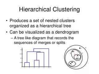
Hierarchicalagglomerativeclustering (HAC) • HAC creates a hierachy in the form of a binary tree. • Assumes a similarity measure for determining the similarity of two clusters. • Start with each document in a separate cluster • Then repeatedly merge the two clusters that are most similar until there is only one cluster • The history of merging is a hierarchy in the form of a binary tree. • The standard way of depicting this history is a dendrogram. 6
A dendrogram • The vertical line of each merger tells us what the similarity of the merger was. • Wecancutthedendrogramat a particularpoint (e.g., at 0.1 or 0.4) to get a flat clustering. 7
Computational complexity of the naive algorithm • First, we compute the similarity of all N × N pairs of documents. • Then, in each of N iterations: • We scan the O(N × N) similarities to find the maximum similarity. • We merge the two clusters with maximum similarity. • We compute the similarity of the new cluster with all other (surviving) clusters. • There are O(N) iterations, each performing a O(N × N) “scan” operation. • Overall complexity is O(N3). • We’ll look at more efficient algorithms later. 9
Key question: How to define cluster similarity • Single-link: Maximum similarity • Maximum similarity of any two documents • Complete-link: Minimum similarity • Minimum similarity of any two documents • Centroid: Average “intersimilarity” • Average similarity of all document pairs (but excluding pairs of docs in the same cluster) • This is equivalent to the similarity of the centroids. • Group-average: Average “intrasimilarity” • Average similary of all document pairs, including pairs of docs in the same cluster 10
Centroid: Averageintersimilarity intersimilarity = similarity of two documents in different clusters 14
Group average: Averageintrasimilarity intrasimilarity = similarity of any pair, including cases where the two documents are in the same cluster 15
Outline • Recap • Introduction • Single-link/ Complete-link • Centroid/ GAAC • Variants • Labeling clusters
Single link HAC • The similarity of two clusters is the maximum intersimilarity – the maximum similarity of a document from the first cluster and a document from the second cluster. • Once we have merged two clusters, we update the similarity matrix with this: • SIM(ωi , (ωk1 ∪ ωk2)) = max(SIM(ωi , ωk1), SIM(ωi, ωk2)) 22
Thisdendogram was producedbysingle-link • Notice: manysmallclusters (1 or 2 members) beingaddedtothemaincluster • Thereisnobalanced 2-cluster or 3-cluster clusteringthatcanbederivedbycuttingthedendrogram. 23
Complete link HAC • The similarity of two clusters is the minimum intersimilarity – the minimum similarity of a document from the first cluster and a document from the second cluster. • Once we have merged two clusters, we update the similarity matrix with this: • SIM(ωi , (ωk1 ∪ ωk2)) = min(SIM(ωi , ωk1), SIM(ωi , ωk2)) • We measure the similarity of two clusters by computing the diameter of the cluster that we would get if we merged them. 24
Complete-link dendrogram • Noticethatthisdendrogramismuchmorebalancedthanthesingle-link one. • Wecancreate a 2-cluster clusteringwithtwoclustersofaboutthe same size. 25
Single-link: Chaining Single-link clustering often produces long, straggly clusters. For most applications, these are undesirable. 28
Complete-link: Sensitivitytooutliers • The complete-link clustering of this set splits d2 from its right neighbors – clearly undesirable. • The reason is the outlier d1. • This shows that a single outlier can negatively affect the outcome of complete-link clustering. • Single-link clustering does better in this case. 29
Outline • Recap • Introduction • Single-link/ Complete-link • Centroid/ GAAC • Variants • Labeling clusters
Centroid HAC • The similarity of two clusters is the average intersimilarity – the average similarity of documents from the first cluster with documents from the second cluster. • A implementation of centroid HAC is computing the similarity of the centroids: • Hence the name: centroid HAC 31
The Inversion in centroidclustering • In an inversion, the similarity increases during a merge sequence. Results in an “inverted” dendrogram. • Below: Similarity of the first merger (d1 ∪ d2) is -4.0, similarity of second merger ((d1 ∪ d2) ∪ d3) is ≈ −3.5. 34
Group-averageagglomerativeclustering (GAAC) • The similarity of two clusters is the average intrasimilarity – the average similarity of all document pairs (including those from the same cluster). • But we exclude self-similarities. • The similarity is defined as: 35
Outline • Recap • Introduction • Single-link/ Complete-link • Centroid/ GAAC • Variants • Labeling clusters
Time complexity of HAC • The algorithm we look at earlier is O(N3). • There is no known O(N2) algorithm for complete-link, centroid and GAAC. • Best time complexity for these three is O(N2 log N). 39
Outline • Recap • Introduction • Single-link/ Complete-link • Centroid/ GAAC • Variants • Labeling clusters
Discriminative labeling • To label cluster ω, compare ω with all other clusters • Find terms or phrases that distinguish ω from the other clusters. • We can use any of the feature selection criteria we introduced in text classification to identify discriminating terms: mutual information. 41
Non-discriminative labeling • Select terms or phrases based solely on information from the cluster itself. • Terms with high weights in the centroid. (if we are using a vector space model) • Non-discriminative methods sometimes select frequent terms that do not distinguish clusters. • For example, MONDAY, TUESDAY, . . . in newspaper text 42
Using titles for labeling clusters • Terms and phrases are hard to scan and condense into a holistic idea of what the cluster is about. • Alternative: titles • For example, the titles of two or three documents that are closest to the centroid. • Titles are easier to scan than a list of phrases. 43
Cluster labeling: Example • Apply three labeling method to a K-means clustering. • Three methods: most prominent terms in centroid, differential labeling using MI, title of doc closest to centroid • All three methods do a pretty good job. 44