Download
1 / 20
431 likes | 1.9k Views
Residual Analysis. Chapter 8. Model Assumptions. Independence (response variables y i are independent)- this is a design issue Normality (response variables are normally distributed) Homoscedasticity (the response variables have the same variance).

E N D
Residual Analysis Chapter 8
Model Assumptions • Independence (response variables yi are independent)- this is a design issue • Normality (response variables are normally distributed) • Homoscedasticity (the response variables have the same variance)
Best way to check assumptions: check the assumptions on the random errors • They are independent • They are normally distributed • They have a constant variance σ2 for all settings of the independent variables (Homoscedasticity) • They have a zero mean. If these assumptions are satisfied, we may use the normal density as the working approximation for the random component. So, the residuals are distributed as: εi ~ N(0,σ2)
Plotting Residuals • To check for homoscedasticity (constant variance): • Produce a scatterplot of the standardized residuals against the fitted values. • Produce a scatterplot of the standardized residuals against each of the independent variables. • If assumptions are satisfied, residuals should vary randomly around zero and the spread of the residuals should be about the same throughout the plot (no systematic patterns.)
Homoscedasticity is probably violated if… • The residuals seem to increase or decrease in average magnitude with the fitted values, it is an indication that the variance of the residuals is not constant. • The points in the plot lie on a curve around zero, rather than fluctuating randomly. • A few points in the plot lie a long way from the rest of the points.
Heteroscedasticity • Not fatal to an analysis; the analysis is weakened, not invalidated. • Detected with scatterplots and rectified through transformation. • http://www.pfc.cfs.nrcan.gc.ca/profiles/wulder/mvstats/transform_e.html • http://www.ruf.rice.edu/~lane/stat_sim/transformations/index.html
Cautions with transformations • Difficulty of interpretation of transformed variables. • The scale of the data influences the utility of transformations. • If a scale is arbitrary, a transformation can be more effective • If a scale is meaningful, the difficulty of interpretation increases
Normality • The random errors can be regarded as a random sample from a N(0,σ2) distribution, so we can check this assumption by checking whether the residuals might have come from a normal distribution. • We should look at the standardized residuals • Options for looking at distribution: • Histogram, Stem and leaf plot, Normal plot of residuals http://statmaster.sdu.dk/courses/st111/module04/index.html
Histogram or Stem and Leaf Plot • Does distribution of residuals approximate a normal distribution? • Regression is robust with respect to nonnormal errors (inferences typically still valid unless the errors come from a highly skewed distribution)
Normal Plot of Residuals • A normal probability plot is found by plotting the residuals of the observed sample against the corresponding residuals of a standard normal distribution N (0,1) • If the plot shows a straight line, it is reasonable to assume that the observed sample comes from a normal distribution. • If the points deviate a lot from a straight line, there is evidence against the assumption that the random errors are an independent sample from a normal distribution. • http://www.skymark.com/resources/tools/normal_test_plot.asp
:Variance of the random errorε • If this value equals zero • all random errors equal 0 • Prediction equation (ŷ) will be equal to mean value E(y) • If this value is large • Large (absolute values) of ε • Larger deviations between ŷ and the mean value E(y). • The larger the value of , the greater the error in estimating the model parameters and the error in predicting a value of y for specific values of x.
Variance is estimated with (MSE) • The units of the estimated variance are squared units of the dependent variable y. • For a more meaningful measure of variability, we use s or Root MSE. • The interval ±2s provides a rough estimation with which the model will predict future values of y for given values of x.
Why do residual analysis? • Following any modeling procedure, it is a good idea to assess the validity of your model. Residuals and diagnostic statistics allow you to identify patterns that are either poorly fit by the model, have a strong influence upon the estimated parameters, or which have a high leverage. It is helpful to interpret these diagnostics jointly to understand any potential problems with the model.
Outliers • What: • An observation with a residual that is larger than 3s or a standardized residual larger than 3 (absolute value) • Why: • A data entry or recording error, Skewness of the distribution, Chance, Unassignable causes • Then what? • Eliminate? Correct? Analyze them? • How much influence do they have? How do I know? • Minitab Storage: Diagnostics (Leverages, Cook’s Distance, DFFITS)
Leverages- p. 403 • Identifies observations with unusual or outlying x-values. • Leverages fall between 0 and 1. A value greater than 2(p/n) is large enough to suggest you should examine the corresponding observation. • p: number of predictors (including constant) • n: number of observations • Minitab identifies observations with leverage over 3(p/n) with an X in the table of unusual observations
Cook’s Distance (D)- p. 405 • An overall measure of the combined impact of each observation on the fitted values. Calculated using leverage values and standardized residuals. Considers whether an observation is unusual with respect to both x- and y-values. • Observations with large D values may be outliers. • Compare D to F-distribution with (p, n-p) degrees of freedom. Determine corresponding percentile. • Less than 20%- little influence • Greater than 50%- major influence
DFFITS- p. 408 • The difference between the predicted value when all observations are included and when the ith observation is deleted. • Combines leverage and Studentized residual (deleted t residuals) into one overall measure of how unusual an observation is • Represent roughly the number of standard deviations that the fitted value changes when each case is removed from the data set. Observations with DFFITS values greater than 2 times the square root of (p/n) are considered large and should be examined. • p is number of predictors (including the constant) • n is the number of observations
Summary of what to look for • Start with the plot and brush outliers • Look for values that stand out in diagnostic measures • Rules of thumb • Leverages (HI): values greater than 2(p/n) • Cook’s Distance: values greater than 50% of comparable F (p, n-p) distribution • DFFITS: values greater than
Let’s do an example • Returning to the Naval Base data set
Finally, are the residuals correlated? • Durbin-Watson d statistic (p. 415) • Range: 0 ≤ d ≤ 4 • Uncorrelated: d is close to 2 • Positively correlated: d is closer to zero • Negatively correlated: d is closer to 4.