Download
1 / 58
610 likes | 811 Views
Testing of Digital Circuits. M. Balakrishnan Dept. of Comp. Sci. & Engg. I.I.T. Delhi. Design Approaches. Test pattern generation to cover a large fraction of the faults Design for testability Built-in-self-test (BIST) Fault tolerant design. Faults: Sources and Types. Sources

E N D
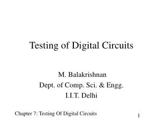
Testing of Digital Circuits M. Balakrishnan Dept. of Comp. Sci. & Engg. I.I.T. Delhi
Design Approaches • Test pattern generation to cover a large fraction of the faults • Design for testability • Built-in-self-test (BIST) • Fault tolerant design
Faults: Sources and Types • Sources • Design process • Device defects • Manufacturing process • Types • Dynamic • Static
Fault Models • Stuck-at faults correspond to a simple fault model • Stuck-at-0 (s-a-0) • Stuck-at-1 (s-a-1) • More complex models are also used but beyond the scope of this work
Combinational Circuits: Test Pattern Generation Problem definition: Given a set of faults (F) and a set of test vectors (T), identify the smallest possible subset of test vectors (V) which covers either all the faults in F or say a predetermined fraction of faults (say 98%).
Fault Simulation Given a test vector, by simulating the circuit with the fault, identify all faults covered by the test vector. Test vectors (T) Faults (F)
Test Generation • Given a fault, identify all the test vectors which can cover that fault. Test vectors (T) Faults (F)
Limitations • Only one fault is expected to occur at one time • Faults other than stuck-at faults are expected to show up as stuck-at faults at some other location • By and large fault location is not possible • These approaches are valid only for combinational circuits
Typical Circuit Enhancements • Insertion of test points • Pin amplification • Test modes • Scan chains
Test Generation Methods M. Balakrishnan Dept. of Comp. Sci. & Engg. I.I.T. Delhi
Parallel Fault Simulation • In parallel fault simulation, evaluation is performed simultaneously for many faults • The number of faults that can be simultaneously simulated corresponds the word length of the host machine
Parallel Fault Simulation (Example) a i b f c h d g e
Deductive Fault Simulation • At each of the primary inputs generate the list of faults that can be detected by the test vector • Use these lists to generate the lists at other nodes by “appropriate” operations on these lists
Deductive Fault Simulation (example) La = {a1} Lb = {b0} Lc = {c1} Ld = {d0} Le = {e1} a 0 i 1 1 b f 0 Lfp = Lb’ Lc = {c1} Lf = {c1, f1} Lgp = (Ld’ Le)’ = {d0} Lg = {d0, g1} Lhp’ = (Lf Lg)’, Lhp = Lh = {h0} Lip’ = La Lh’, Lip = {h0} Li = {h0, i0} c h 0 1 1 0 d g 0 e
Deductive Fault Simulation(example contd.) La = {a1} Lb = {b0} Lc = {c0} Ld = {d0} Le = {e1} a 0 i 1 1 b f 1 Lfp’ = Lb’ Lc’ = { b0, c0} Lf = {b0, c0, f0} Lgp = (Ld’ Le)’ = {d0} Lg = {d0, g1} Lhp’ = (Lf ‘ Lg)’ Lhp = {d0,g1} , Lh = {d0,g1,h0} Lip’ = La Lh’, Lip = {d0, g1,h0} Li = {d0, g1, h0, i0} c h 1 1 1 0 d g 0 e
Test Generation Methods Boolean Difference & D-Algorithm M. Balakrishnan Dept. of Comp. Sci. & Engg. I.I.T. Delhi
Boolean Difference Consider a function f of say 4 variables f(x0, x1, x2, x3) Boolean difference of f w.r.t to xi is defined as follows: df/dxi = fxi=0 + fxi=1
Boolean Difference (example) a i b f c h d g i = a + ((b.c). (d +e)’)’ e di/da = ia=0 + ia=1 = ((b.c).(d+e)’)’ + 1= (b.c)(d+e)’
Example (contd.) di/da = (b.c)(d+e)’ s-a-0 fault at a can be tested by a.di/da = 1 or a.b.c(d+e)’ = 1 test vectors (1,1,1,0,0) s-a-1 fault at a can be tested by a’.di/da = 1 or a’.b.c(d+e)’ = 1 test vectors (0,1,1,0,0)
Boolean Difference (contd.) a b f c h d g i = a + (f. (d +e)’)’ e di/df = if=0 + if=1 = 1 + (a +d+e) = (a+d+e)’ = a’d’e’
Boolean Difference (contd.) di/df = a’.d’.e’ s-a-0 fault at f can be tested by f.di/df = 1 or fa’d’e’ = b.c.a’d’e’ =1 test vectors (0,1,1,0,0) s-a-01fault at f can be tested by f’.di/df = 1 or f’.a’d’e’ = (b.c)’.a’d’e’ = 1 test vectors (0,0,X,0,0) and (0, X,0,0,0)
D-Algorithm There are three main steps in the D-Algorithm • Generate the fault • Propagate the fault to one of the outputs (Forward or D-Drive) • Back propagate to get consistent assignment for inputs (Backward drive or back-propagation)
D-Algorithm (Step 1) a i 4 b f 1 c h 3 d g Let us say we choose the fault g node s-a-0 2 e Assign inputs to gate 2 to generate the fault i.e. d = 0 and e = 0
D-Algorithm (Step 2) a i 4 b f 1 c h 3 0 D d g Choose a path to the o/p and propagate the fault 0 2 e f is to be assigned 1 and a is to be assigned 0 to propagate D to the output i
D-Algorithm (Step 3) 0 a D’ i 4 b f 1 c D’ h 1 3 0 D d g Consistency Check 0 2 e Assign inputs to gates (whose outputs have been specified ) consistent with other assignments
D-Algorithm Result 0 a D’ i 4 1 b f 1 c D’ h 1 1 3 0 D d g 0 2 e The test vector is (0,1,1,0,0)
D-Algorithm M. Balakrishnan Dept. of Comp. Sci. & Engg. I.I.T. Delhi
Terminology • Singular Cover • D-intersection • Primitive D-cube of a fault (pdcf) • Propagation D-cubes (pdf)
Singular Cover SC of a gate (or any circuit element) is nothing but a compact version of the truth table. SC of a AND gate with a and b as inputs and c as output a b c 0 X 0 X 0 0 1 1 1
Singular Cover (contd.) SC of a NOR gate with a and b as inputs and c as output a b c 1 X 0 X 1 0 0 0 1
Primitive D-Cube of Fault (pdcf) For generating a s-a-0 fault at node c, choose a SC row which gives an o/p of 1 for the nor gate and intersect with (X,X,0). pdcf is (0, 0, D) a c b
PDCF (contd.) For generating a s-a-1 fault at node c, choose a SC row which gives an o/p of 0 for the nor gate and intersect with (X,X,1). pdcf is (1, X, D) or (X, 1, D) a c b
Propagation D-Cube (pdc) • PDC consists of a table for each circuit element which has entries for propagating faults on any one of its inputs to the output. • To generate PDC entry corresponding to any one column, D-intersect any two rows of SC which have opposite values (0 and 1) in that column. • There can be multiple rows for one column
PDC Example PDC of a AND gate with a and b as inputs and c as output a b c 1 D D D 1 D
PDC Example (contd.) PDC of a NOR gate with a and b as inputs and c as output a b c 0 D D’ D 0 D’
D-Algorithm Steps • Choose a stuck-at-fault at any of the nodes. • Choose a pdcf for generating the fault. • Choose an output and a path to the output and propagate the fault to the output by choosing pdc for all circuit elements on the path. (D-Drive) • Use the SC of all unassigned circuit elements to arrive at a consistent set of inputs. (back-propagate or consistency check)
D-Algorithm: PDCF Example a i 4 b f 1 c h 3 d g 2 e Choose a fault say g s-a-0. Choose pdcf of gate 2 for generatingthis fault (a b c d e f g h i ) = (X X X 0 0 X D X X)
D-Algorithm: D-Drive Example Propagate the fault to the o/p using pdc of gates 3 &4 a i 4 b f 1 c h 3 0 D d g pdc 3 (X X X 0 0 1 D D’ X) pdc 4 (0 X X 0 0 1 D D’ D’) 0 2 e
D-Algorithm: Consistency Example Perform consistency operation for gate 1 a i 4 b f 1 c h 3 0 D d g (X X X 0 0 1 D D’ X) sc 1 (0 1 1 0 0 1 D D’ D’) 0 2 e
Testing of Sequential Circuits M. Balakrishnan Dept. of Comp. Sci. & Engg. I.I.T. Delhi
Testing Techniques • State table verification • Random testing • Transition count testing • Scan based testing • Signature analysis
State Table Verification Verify each transition by first taking the machine to a specific initial state, applying the input to perform the transition and then verifying the final state. For this purpose we need a homing sequence and distinguishing sequence
Homing & Distinguishing Sequence • Homing sequence: An input is said to be a homing sequence for a m/c if the m/c’s response to the sequence is always sufficient to determine uniquely its final state. • Distinguishing sequence: An input sequence which when applied to a machine will produce a different output sequence for each choice of initial state.
Example: Homing Sequence (ABCD) 1 0 (ABCD) (AB)(D) 0 1 (BD)(C) (AB)(D) 1 0 (BC)(A) (A)(D)(D)
Random Testing Circuit under test Random pattern generator Compare Known good ckt
Transition Count Testing • Count the number of transitions for a specific input pattern and compare with the value stored for “good” circuits • Reduction in data storage for storing correct responses • “Aliasing” errors