Download
1 / 43
450 likes | 673 Views
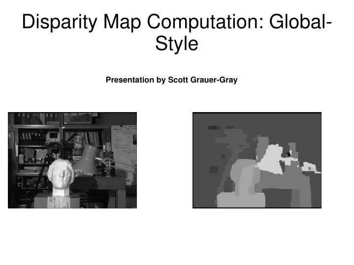
Disparity Map Computation: Global-Style. Presentation by Scott Grauer-Gray. Stereo Overview. Given a reference image and matching (test) image Goal is to find the disparity between each pixel in the reference image and the corresponding pixel in the matching (test) image

E N D
Disparity Map Computation: Global-Style Presentation by Scott Grauer-Gray
Stereo Overview • Given a reference image and matching (test) image • Goal is to find the disparity between each pixel in the reference image and the corresponding pixel in the matching (test) image • Disparity is inversely proportional to depth • Objects with greater disparity --> closer to “cameras”/ “eyes” (or wherever the image is from) • Objects with smaller disparity --> farther from “cameras” / “eyes” (or wherever the image is from)
Calculating the Disparity Map • Many algorithms/papers published on topic • Overview and evaluation of algorithms: A Taxonomy and Evaluation of Dense Two-Frame Stereo Correspondence Algorithms • Current evaluation at http://vision.middlebury.edu/stereo/
Stereo Assumptions • Surface assumptions • Surfaces in image are Lambertian...appearance does not vary with viewpoint • Surfaces are piece-wise smooth; disparity of a single surface does not randomly “jump” around • Camera calibration/epipolar geometry • Pair of rectified images given as input
Calculating Disparity Maps • Most stereo correspondence algorithms use all or some of following steps • Matching cost computation • Cost (support) aggregation • Disparity computation/optimization • Disparity refinement
Matching Cost Computation • Matching Cost Computation – cost of matching point (x1, y1) in reference image to point (x2, y2) in test image • In SSD algorithm, matching cost = squared difference of intensity values of pixels at disparity d • Other matching costs: sum of absolute difference (SAD), normalized cross-correlation (NCC), Birchfield-Tomasi
Cost (support) aggregation • Cost (support) aggregation – summing the costs of matching pixels in a given region (possibly using weights) • In SSD algorithm, aggregation is performed by averaging together matching costs for each pixel within a window at each given disparity using a box filter • Aggregation can be performed using a Gaussian/ binomial filter to provide greater weight to pixels near center of window
Disparity Computation/optimization • Retrieves calculated disparity at each pixel in reference image, method varies by algorithm • In SSD algorithm, uses “winner-take-all” method • Inspects aggregated cost associated with each disparity via window centered around pixel • Disparity with the smallest aggregated cost is selected • Step can be performed “in parallel” for every pixel in the reference image
Disparity Refinement • Disparity estimates generally in discretized space (such as integer pixel values) • Some algorithm have refinement step to compute sub-pixel disparities after initial computations • Methods include iterative gradient descent and fitting a curve to matching costs at discrete disparity levels • Alternative is starting with more disparity levels
Stereo Algorithms • Most stereo algorithms can be placed one of two categories • Local – disparity computation dependent on intensity values within finite window in reference and matching (test) image; smoothness assumption is implicit with aggregating support • Global – stereo matching problem converted to global function; goal to optimize this global function that (likely) combines matching cost and smoothness cost terms (and possibly others...); smoothness assumption encoded explicitly
Local Stereo • Example: SSD using fixed windows • One problem: setting correct size of window • Small window: may not be enough intensity variation; signal to noise ratio low • Large window: may cover region with multiple disparities • Paper by Kanade referenced in previous lecture goes into more detail about this... • Another problem: what about texture-less regions?Aggregated matching cost near 0 for multiple disparities
Global Stereo • Goal is to retrieve disparity map that optimizes a global function • Global function can vary across different global algorithms/implementations • Matching cost of corresponding pixels in ref/test images given disparity often encoded into function • Function often contains a “smoothness cost” - explicitly encodes the “piecewise smooth” assumption • Smoothness cost compares computed disparities of neighboring pixels in disparity map (greater difference in disparity -> greater smoothness cost)
Global Stereo: MRF • Global method: formulate stereo matching problem as a Markov network • Markov network - Probabilistic graph model • Undirected graph of n nodes with pairwise potentials (given by compatibility function...) • State of each node i represented as x_i • Given some “evidence” Y • Joint compatibility function: ϕ(x_s, Y) • Output can be considered “evidence” for x_s given Y; greater if x_s is more likely • Compatibility function: ψ(x_s, x_t) • Encodes “pairwise potential”/compatibility between neighboring nodes x_s, x_t; small if node pair not “compatible”
Global Stereo: MRF • Goal: retrieve “most likely” set of nodes { x_1, x_2, ..., x_n} given the evidence Y and the compatibility between neighboring nodes • Joint probability distribution function of n nodes: • P( x_1, x_2, ..., x_n | Y) = Π ϕ(x_s, Y) Πψ(x_s, x_t) All nodes s All “neighboring” nodes s, t • Target: retrieve set of nodes that maximizes joint probability distribution
Global Stereo: MRF • Target: turn stereo matching problem into Markov random field problem • Given: stereo set of images • Color/intensity values of pixels in stereo images can be viewed as the “evidence” • Current goal: Find the disparity map that maximizes P(disparity map | stereo set) • No obvious solution... • However, you do have some idea of P( stereo set | disparity map) and P(disparity map) • How can you use this information?
Global Stereo: MRF • Bayes rule: P( X | Y) = (P( Y | X) * P(X)) / P(Y) • Using Bayes rule... • P(disparity map | stereo set) = (P(stereo set | disparity map) * P(disparity map)) / (P(stereo set)) • Given stereo set --> P(stereo set) can be set to 1.0f • Now, P(disparity map | stereo set) = P(stereo set | disparity map) * P(disparity map) • New Goal: retrieve disparity map that maximizes P(stereo set | disparity map) * P(disparity map) • One of these terms can be viewed as encoding the “matching” cost/probability with the other one encoding smoothness of the disparity map... • Which one is which?
Global Stereo: MRF • Target: retrieve P(stereo set | disparity map) • Probability represents total matching cost across all pixels in a stereo set given the disparity map • Greater total matching cost --> lower P(stereo set | disparity map) • If matching cost of every pixel is 0 given the current disparity map, then P(stereo set | disparity map) = 1 • matching costs of pixels increase -> P(stereo set | disparity map) decreases • If matching cost of any pixel is infinity --> assume P(stereo set | disparity map) = 0 • Can use property to rule out certain disparity maps
Global Stereo: MRF • P(stereo set | disparity map) = Π (e^((-1) * matching cost of s given d_s in disp. map)) All pixels s in disparity map • Value of P(stereo set | disparity map) is between 0-1 inclusive • If matching cost of all pixels is 0, P(stereo set | disparity map) = 1 since e^0 = 1 • If matching cost of any pixel is infinity P(stereo set | disparity map) = 0 since e^(-infinity) = 0 • As matching costs of pixel(s) increase, P(stereo set | disparity map) decreases
Global Stereo: MRF • Target: retrieve P(disparity map) • Represents total smoothness cost of disparity map • Smoothness cost and P(disparity map) are inversely related (why...remember goal is to minimize smoothness cost) • Assume that pixels near each other have the same disparity --> smoothness cost increases when this condition is violated • Case where all pixels have same disparity -> total smoothness cost is 0 -> P(disparity map) = 1 • Smoothness cost approaches infinity -> P(disparity map) approaches 0
Global Stereo: MRF • How to compute smoothness cost? • One method: use function that takes disparities of neighboring pixels in disparity map (generally 4-connected neighbors used) • If neighboring pixels have same disparity -> cost is 0 • Cost increases as change in disparity (between neighboring pixels) increases • What to do about discontinuities? • May want to account for them in some manner • Could truncate smoothness cost at some point...prevent large jumps in disparity from being over-penalized • Could use segmentation (in pre-processing) to encode discontinuities and set smoothness cost to 0 where discontinuities expected...(this goes beyond basic stereo)
Global Stereo: MRF • P(disparity map) = Π (e^((-1) * smoothness cost between s and t given d_s and d_t)) All 4-connected neighboring pixels s, t in disparity map • If smoothness cost of all sets of neighboring pixels is 0, P(disparity map) = 1 • If smoothness cost of any set of neighboring pixels is infinity --> P(disparity map) = 0 • Note that stereo image set has nothing to do with this probability • Disparity of all pixels in disparity map = constant c --> P(disparity map) = 1 (regardless of stereo set...)
Global Stereo: MRF • Original goal: maximize P(disparity map | stereo set) • Used Bayes to set P(disparity map | stereo set) = P(stereo set | disparity map) * P(disparity map) • Using new info... • P(disparity map | stereo set) = Π (e^((-1) * matching cost of s given d_s in disp. map and stereo set)) * All pixels s in disparity map Π (e^((-1) * smoothness cost between s and t given d_s and d_t)) All 4-connected neighboring pixels s, t in disparity map
Global Stereo: MRF • Models for matching cost • Same as local window: SAD, SSD, NCC, Birchfield-Tomasi -> use corresponding pixels in ref/test images for given disparity to compute cost • Models for smoothness cost • Linear model commonly used: analogous to SAD for matching cost • Smoothness cost between neighboring pixels on disparity map = absolute difference in disparity • Linear model often truncates disparity difference at a given value to allow for discontinuities without too large of a penalty • Other models: Potts model, quadratic model
Global Stereo: MRF • Retrieving P( stereo set | disparity map ) and P(disparity map) in “toy” stereo sets • See next few slides... • Assume that SAD model used for matching cost computation • Assume linear model in smoothness cost computation • What would be the “simplest” possible stereo set?
Global Stereo: MRF • Toy stereo set #1: • Two all “black” images given as stereo set • What will be the P(stereo set | disparity map) when all disparities are 0? • What will be P(disparity map) when all disparities are 0? • What is P(disparity map | stereo set) when disparities = 0? • Will P(stereo set | disparity map) change if disparity map changes?
Global Stereo: MRF • Toy Stereo Set #2: • Two identical images given as stereo set (Tsukuba reference image, as an example) • What will be the P(stereo set | disparity map) when all disparities are 0? • What will be P(disparity map) when all disparities are 0? • Will P(stereo set | disparity map) change if disparity map changes? • What happens when all disparities = 1 in disparity map?
Global Stereo: MRF • Toy Stereo set #3: Grayscale stereo set with textured “background” and black object “foreground” • Disparity of textured “background” is 0 • Disparity of “black” object is 5 • Given ground truth disparity map... • What will be the P(stereo set | disparity map) when all disparities are 0? • What will P(stereo set | disparity map) when all disparities correspond to ground truth? • What will be P(disparity map) when all disparities are 0? • What will be P(disparity map) when all disparities correspond to ground truth? Ref Image Ground truth disparity map
Global Stereo: MRF • Back to the Markov Random Field... • Markov network - undirected graph of n nodes with pairwise potentials • State of each node i -> x_i • Given “evidence” Y • Joint probability distribution function of nodes: • P( x_1, x_2, ..., x_n | Y) = Π ϕ(x_s, Y) Π ψ(x_s, x_t) All nodes s All “neighboring” nodes s, t
Global Stereo: MRF • Stereo... • Find disparity map to maximize P(disparity map | stereo set) where P(disparity map | stereo set) = Π (e^((-1) * matching cost of s given d_s in disp. map)) * All pixels s in disparity map Π (e^((-1) * smoothness cost between s and t given d_s and d_t)) All 4-connected neighboring pixels s, t in disparity map • MRF... • Find set of n nodes with states x_1, x_2, ..., x_n needed to maximize P(x_1, x_2, ..., x_n | Y) = • Y = local “evidence” Π ϕ(x_s, Y) Π ψ(x_s, x_t) All nodes s All “neighboring” nodes s, t
Global Stereo: MRF • Maximizing P(disparity map | stereo set): equivalent to maximizing P(x_1, x_2, ..., x_n | Y) in Markov network • Set of states x_1, x_2, ..., x_n in Markov network --> set of pixels in disparity map, each with a disparity value (assigned disparity value = “state”) • “Evidence” Y in Markov network --> given stereo set of images • (A) mission accomplished: stereo problem turned into Markov network problem • Specifically, the stereo problem has been “reduced to” retrieving the maximum a posteriori (MAP) estimation in the Markov network
Global Stereo: MRF • Retrieving the MAP estimation in the Markov network • NP-complete problem; often infeasible to solve using “brute force” • Each pixel (“node”) in disparity map can take any value in disparity space (“state”) • Methods used to estimate solution in reasonable amount of time • Graph cuts • Belief propagation
Global Stereo: MRF • Belief Propagation • Iterative inference algorithm that can be used on Markov network problems • Works by sending messages through the network for a number of iterations • Eventually, the message values at each node will converge and then the message values are used to retrieve the estimated state of the node • Retrieves optimal solution in graphs without loops • Called loopy belief propagation in graphs with loops (such as graph resulting from stereo problem) • No guarantee of optimal solution, but generally gives a good approximation
Belief Propagation • Can be used to retrieve the MAP estimation in the Markov network • Each node computes messages to send to four-connected neighbors • Each message can be viewed as a vector containing a value for each possible disparity • Messages are computed at each pixel (in each iteration) and then passed to four-connected neighbors • Messages computed using data cost and message values from neighbors (computed in previous iteration) • Higher message value --> higher probability of corresponding disparity
Belief Propagation: Message Computation • Messages initially initialized to 1 • Message from pixel s to neighbor t in iteration i+1 corresponding to disparity d_x computed via: i+1 i+1 i M_st(d_x) = max( Ψ(d_x, d_y) * ϕ(d_x, Y) * Π M_ks(d_y) d_y in disparity space All neighbors k of s except t Computational running time for each message at each pixel: O(D^2), where D is the size of the disparity space • Message values will converge after “enough” iterations • Once message values converge, message values (with joint compatibility function) used to compute estimated disparity at each pixel
Belief Propagation • After all BP iterations complete... • Compute belief value of each disparity d_x at each pixel s • b_s(d_x) = ϕ(d_x, Y) * Π M_ks(d_x) All neighbors k of s • Disparity value at each pixel in disparity map is set to d_x corresponding to the maximum belief value • Resulting disparity map is estimation of desired disparity map that maximizes P(disparity map | stereo set) from the original problem via the MRF formulation and the MAP estimation • We are done! (or are we...)
Belief Propagation: Analysis • Results for Tsukuba stereo set: Result using window-based matching: Reference image: Result using Belief propagation: Ground truth:
Running time of Belief Propagation • Algorithm runs for I iterations • D values in disparity space • Images in stereo set are of size N * M • Total Running time (sequential): • Computation of data costs: O(N*M*D) • Computation of computing/passing message values in each iteration (naive): O(N*M*D^2) • Computation of calculated disparity values: O(N*M*D) • Total running time = O(N*M*D) + I * O(N*M*D^2) * O(N*M*D) = O(N*M*I*D^2) • Running time if computations performed on all pixels in parallel?
Storage requirements of Belief Propagation • Initially: need to store the 2 N*M images in stereo set: O(2*N*M) (not needed after data costs computed) • Matching cost stored for every pixel at each disparity: O(N*M*D) • Four message vectors of size D stored for every pixel: O(4*N*M*D) • Total storage requirement: O(5*N*M*D)
Advantages of Belief Propagation • Resulting disparity map is close to minimization of data and smoothness costs • Resulting disparity map relatively accurate in practice • Generally better results than local methods such as SSD (even if adaptive windows are used) • Can be extended to incorporate occlusion, segmentation, and other info to further improve the results • The #2 and #3 stereo algorithms according to the Middlebury benchmark are based on belief propagation
Drawbacks of Belief Propagation • Requires many iterations for message values to converge and retrieve an accurate disparity estimate • High storage requirements
Drawbacks of Belief Propagation • Felzenwalb (2004) presents methods to account for these drawbacks • Hierarchical scheme to reduce number of iterations -> longer-range interactions between pixels in fewer iterations course levels • Checkerboard scheme for message passing • Only half of the pixels must compute message values in each iteration • Allows BP iterations to be performed in place; cuts storage requirements
Other Global Methods • Belief propagation's primary “competitor” is graph cut • Either can be used to minimize total data and smoothness costs in global function • Tappan (2003) compared the two algorithms using identical parameters • Disparity maps retrieved using graph cut had slightly lower energy, but results similar in relation to ground truth • Belief propagation appears more popular based on Middlebury benchmark evaluation