Download
1 / 33
330 likes | 418 Views
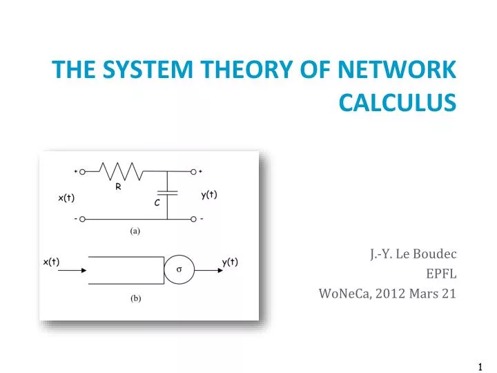
J.-Y. Le Boudec EPFL WoNeCa , 2012 Mars 21. The System Theory of Network Calculus. Contents. Network Calculus’s System Theory and Two Simple Examples More Examples Time versus Space. The Shaper. fresh traffic. shaped traffic s -smooth. s. R. R*.

E N D
J.-Y. Le Boudec EPFL WoNeCa, 2012 Mars 21 The System Theory of Network Calculus 1
Contents • Network Calculus’s System Theoryand Two Simple Examples • More Examples • Time versus Space 2
The Shaper fresh traffic shaped traffic s-smooth s R R* • shaper: forces output to beconstrained by • greedyshaperstoresdata in a buffer only if needed • examples: • constant bit rate link (s(t)=ct) • ATM shaper; fluidleakybucketcontroller • Pb: find input/output relation 3
A Min-Plus Model of Shaper fresh traffic shaped traffic s-smooth s R x • Shaper Equations: (1) (2) • and are functions • issub-additive • is min-plus convolution 4
Network Calculus’s System Theory • = set offunctions that are wide-sense increasing • Also works in continuous time, functions are left-continuous • An operator is a mapping : G -> G • is isotone if x(t)y(t)(x)(t) (y)(t) • is upper-semi continuousiffinfi((xi )) = (infi(xi)) for sequences xi 5
Min-Plus Linear Operators • is min-plus linear if • for any constant K, (x + K) = (x) + K (x y) = (x) (y) • is upper-semi continuous. • Representation Theorem: is min-plus linear <=>there is a unique H: R x R -> R+ , in and in , such that (x)(t)=infs[H(t,s)+x(s)] • min-plus linear => isotone and upper semi-continuous • Example: convolution operator • Example: isgiven: 6
Min-Plus ResiduationTheorem Theorem: ([L., Thiran 2001]thm 4.3.1., derived from Baccelli et al., ) Assume that is isotone and upper-semi-continuous. Theproblem x(t)b(t) (x)(t) where is the unknown functionhas one maximum solution in , given by x*(t)= (b)(t) • (Definition of closure) (x) = inf {x, (x), (x), (x),...} • in other words: x0 = b ; xi = (xi-1) and x* = inf {x0, x1, ..., xi, ...} 7
(1) x x (2)x R Application to Shaper fresh traffic shapedtraffic s-smooth s R R* • There is a maximum solution obtained by iteratingbecauseThus • The greedyshaper output is R*= R • , the subadditiveclosure of is 8
Variable CapacityNode fresh traffic m(t) R R* • node has a time varyingcapacityµ(t)Define M(t) =0tm(s) ds. • the output satisfies R*(t) R(t) R*(t) -R*(s) M(t) -M(s) for all s tand is “as large as possible” 9
Variable CapacityNode fresh traffic m(t) R R* • Operator : s.t. • We have the problem • and the sub-additive closure of is • There is a maximum solution, R*(t) R(t) R*(t) -R*(s) M(t) -M(s) for all s t 10
2. MORE examples 11
A System withLoss[Chuang and Cheng 2000] Loss L(t) fresh traffic R(t) b R’(t) buffer X R*(t) • node with service curve b(t) and buffer of size X • when buffer is full incoming data is discarded • modelled by a virtual controller (not buffered) • fluid model or fixed sized packets • Pb: find loss ratio 12
A System withLoss Loss L(t) fresh traffic R(t) b R’(t) buffer X R*(t) • Assume is smooth; if then no loss • If , whatcanwesay ? (t) 13
Bound on Loss Ratio Loss L(t) fresh traffic R(t) b R’(t) buffer X R*(t) • Thm[Chuang and Cheng 2000] Let be the largestsuchthat i.e. Then; itis thebest possible bound. (t) (t) 14
Analysis of System withLoss Loss L(t) fresh traffic R(t) b R’(t) buffer X R*(t)= • (splitter) • (buffer does not overflow) where is the transformation R’ -> R, assumed isotone and usc (« physical assumptions ») • There is a maximum solution and R’ is the maximum solution 15
Analysis of System withLoss Loss L(t) fresh traffic R(t) b R’(t) buffer X R*(t)= • Let withgiven by thm. • Eqn 1 issatisfied • is smooth, thus required buffer and Eqn 2 is satisfied • Thus and 16
Optimal Smoothing[L.,Verscheure 2000] Video server Video display Network Smoother R(t) R’(t) R*(t) R(t-D) ß(t) B s • Network + end-client offer a service curve b to flow R’(t) • Smoother delivers a flow R’(t) conforming to an arrival curve s. • Video stream is stored in the client buffer, read after a playback delay D. • Pb: which smoothing strategy minimizes D? 17
Optimal Smoothing, System Equations Video server Video display Network Smoother R(t) R’(t) R*(t) R(t-D) ß(t) B s • (1) R’ is s-smooth(2) (R’(t) R(t-D) • Use deconvolution)= x y <=> x y • system becomes(1) R’ R’ s (2)R’ (R )(t-D) 18
Optimal Smoothing, System Equations Video server Video display Network Smoother R(t) R’(t) R*(t) R(t-D) ß(t) B s • This is a max-plus linear problem, it has a minimum solution given by the iterations:(R ( ))(t-D) because • Thus 19
Example s b(t) * 106 5 4 3 2 1 a possible R’(t) R(s b)(t-D) -50 0 50 100 150 200 250 300 350 400 450 Frame # R(t-D) 20
Minimum Playback Delay • D must satisfy :R ( s) (-D) 0 • thisisequivalent to D h(R, s) 21
R(t) 70 10000 60 50 40 8000 30 D = 435 ms 20 10 6000 100 200 300 400 (s b)(t) (s b)(t) 4000 2000 100 200 300 400 10000 D = 102 ms 70 8000 60 6000 50 40 4000 30 2000 20 10 100 200 300 400 100 200 300 400 22
The PerfectBattery • Battery maybecharged ()or discharged () • Loadisgiven • Problemis to determine a power schedule , subject to and withinbatteryconstraints 23
System Equations for the PerfectBattery • no underflow • no overflow • power constraint where are cumulative functionssuch as 24
System Equations • Relax (eq 1): There is a maximum solution, is causal The problemisfeasibleiffsatisfies (eq 1), i.e. no underflow no overflow 25
System Equations • Relax (eq 2):There is a minimum solution, is non-causal The problemisfeasibleiffsatisfies (eq 2)This gives the same conditions no underflow no overflow 26
3. TIME versus Space 27
The ResiduationTheoremis a SpaceMethod • The maximum solution to the problemisgiven by iterates over the entiretrajectory • When time isdiscretetheremaybeanotherway to compute by time recursion 28
(1) x x (2)x R The Shaper, Time Method fresh traffic shapedtraffic s-smooth s R R* • Time isdiscrete • Defineby: • is solution • For anyother solution , [induction] • is the maximal solution, i.e. • Note the difference in representation: 29
The Time Method for LinearProblems • [L., Thiran 2001] Thm 4.4.1: the problem in discrete timewhere, in and in has a maximal solution given by • This is a second, alternative representationfor 30
PerfectBattery There is a maximum solution, It canbecomputedby the time method: The minimum scheduleis anti-causal and canbecomputedwith time reversal 31
Conclusion • Min-plus and max-plus system theorycontains a central result : residuationtheorem ( = fixed point theorem)Establishes existence of maximum (resp. minimum) solutionsand provides a representation • Space and Time methodsgivedifferentrepresentations 32
Thank You… 33