Download
1 / 48
480 likes | 645 Views
National Accounts and SAM Estimation Using Cross-Entropy Methods. Sherman Robinson. Estimation Problem. Partial equilibrium models such as IMPACT require balanced and consistent datasets the represent disaggregated production and demand by commodity

E N D
National Accounts and SAM Estimation UsingCross-Entropy Methods Sherman Robinson
Estimation Problem • Partial equilibrium models such as IMPACT require balanced and consistent datasets the represent disaggregated production and demand by commodity • Estimating such a dataset requires an efficiency method to incorporate and reconcile information from a variety of sources
Primary Data Sources for IMPACT Base Year • FAOSTAT for country totals for: • Production: Area, Yields and Supply • Demand: Total, Food, Intermediate, Feed, Other Demands • Trade: Exports, Imports, Net Trade • Nutrition: Calories per capita, calories per kg of commodity • AQUASTAT for country irrigation and rainfed production • SPAM pixel level estimation of global allocation of production
Information Theory Approach • Goal is to recover parameters and data we observe imperfectly. Estimation rather than prediction. • Assume very little information about the error generating process and nothing about the functional form of the error distribution. • Very different from standard statistical approaches (e.g., econometrics). • Usually have lots of data
Estimation Principles • Use all the information you have. • Do not use or assume any information you do not have. • Arnold Zellner: “Efficient Information Processing Rule (IPR).” • Close links to Bayesian estimation
Information Theory • Need to be flexible in incorporating information in parameter/data estimation • Lots of different forms of information • In classic statistics, “information” in a data set can summarized by the moments of the distribution of the data • Summarizes what is needed for estimation • We need a broader view of “estimation” and need to define “information”
initial state of motion. final state of motion. Force is whatever induces a change of motion: An analogy from physics Force
old beliefs new beliefs Inference is dynamics as well information “Information” is what induces a change in rational beliefs.
Information Theory • Suppose an event E will occur with probability p. What is the information content of a message stating that E occurs? • If p is “high”, event occurrence has little “information.” If p is low, event occurrence is a surprise, and contains a lot of information • Content of the message is not the issue: amount, not meaning, of information
Information Theory • Shannon (1948) developed a formal measure of “information content” of the arrival of a message (he worked for AT&T)
Information Theory • For a set of events, the expected information content of a message before it arrives is the entropy measure:
E.T. Jaynes • Jaynes proposed using the Shannon entropy measure in estimation • Maximum entropy (MaxEnt) principle: • Out of all probability distributions that are consistent with the constraints, choose the one that has maximum uncertainty (maximizes the Shannon entropy metric) • Idea of estimating probabilities (or frequencies) • In the absence of any constraints, entropy is maximized for the uniform distribution
Estimation With a Prior • The estimation problem is to estimate a set of probabilities that are “close” to a known prior and that satisfy various known moment constraints. • Jaynes suggested using the criterion of minimizing the Kullback-Leibler “cross entropy” (CE) “divergence” between the estimated probabilities and the prior.
Cross Entropy Estimation “Divergence”, not “distance”. Measure is not symmetric and does not satisfy the triangle inequality. It is not a “norm”.
MaxEnt vs Cross-Entropy • If the prior is specified as a uniform distri-bution, the CE estimate is equivalent to the MaxEnt estimate • Laplace’s Principle of Insufficient Reason: In the absence of any information, you should choose the uniform distribution, which has maximum uncertainty • Uniform distribution as a prior is an admission of “ignorance”, not knowledge
Cross Entropy Measure • Two kinds of information • Prior distribution of the probabilities • Moments of the distribution • Can know any moments • Can also specify inequalities • Moments with error will be considered • Summary statistics such as quantiles
Cross-Entropy (CE) Estimates • Ω is called the “partition function”. • Can be viewed as a limiting form (non-parametric) of a Bayesian estimator, transforming prior and sample information into posterior estimates of probabilities. • Not strictly Bayesian because you do not specify the prior as a frequency function, but a discrete set of probabilities.
From Probabilities to Parameters • From information theory, we now have a way to use “information” to estimate probabilities • But in economics, we want to estimate parameters of a model or a “consistent” data set • How do we move from estimating probabilities to estimating parameters and/or data?
Types of Information • Values: • Areas, production, demand, trade • Coefficients: technology • Crop and livestock yields • Input-output coefficients for processed commodities (sugar, oils) • Prior Distribution of measurement error: • Mean • Standard error of measurement • “Informative” or “uninformative” prior distribution
Data Estimation • Generate a prior “best” estimate of all entries: Values and/or coefficients. • A “prototype” based on: • Values and aggregates • Historical and current data • Expert Knowledge • Coefficients: technology and behavior • Current and/or historical data • Assumption of behavior and technical stability
Estimation Constraints • Nationally • Area times Yield = Production by crop • Total area = Sum of area over crops • Total Demand = Sum of demand over types of demand • Net trade = Supply – Demand • Globally • Net trade sums to 0
Measurement Error • Error specification • Error on coefficients or values • Additive or multiplicative errors • Multiplicative errors • Logarithmic distribution • Errors cannot be negative • Additive • Possibility of entries changing sign
Error Specification • Errors are weighted averages of support set values • The v parameters are fixed and have units of item being estimated. • The W variables are probabilities that need to be estimated. • Convert problem of estimating errors to one of estimating probabilities.
Error Specification • The technique provides a bridge between standard estimation where parameters to be estimated are in “natural” units and the information approach where the parameters are probabilities. • The specified support set provides the link.
Error Specification • Conversion of a “standard” stochastic specification with continuous random variables into a specification with a discrete set of probabilities • Golan, Judge, Miller • Problem is to estimate a discrete probability distribution
Uninformative Prior • Prior incorporates only information about the bounds between which the errors must fall. • Uniform distribution is the continuous uninformative prior in Bayesian analysis. • Laplace: Principle of insufficient reason • We specify a finite probability distribution that approximates the uniform distribution.
Uninformative Prior • Assume that the bounds are set at ±3s where s is a constant. • For uniform distribution, the variance is:
Uninformative Prior • Finite uniform prior with 7-element support set is a conservative uninformative prior. • Adding more elements would more closely approximate the continuous uniform distribution, reducing the prior variance toward the limit of 3s2. • Posterior distribution is essentially unconstrained.
Informative Prior • Start with a prior on both mean and standard deviation of the error distribution • Prior mean is normally zero. • Standard deviation of e is the prior on the standard error of measurement of item. • Define the support set with s=σ so that the bounds are now ±3σ.
Informative Prior, 2 Parameters Mean Variance
Informative Prior: 4 Parameters • Must specify prior for additional statistics • Skewness and Kurtosis • Assume symmetric distribution: • Skewness is zero. • Specify normal prior: • Kurtosis is a function of σ. • Can recover additional information on error distribution.
Informative Prior, 4 Parameters Mean Variance Skewness Kurtosis
Implementation • Implement program in GAMS • Large, difficult, estimation problem • Major advances in solvers. Solution is now robust and routine. • CE minimand similar to maximum likelihood estimators. • Excel front end for GAMS program • Easy to use