Download
1 / 32
330 likes | 497 Views
Benefit Estimation Methods. Andrew Foss ( andrew_foss@ksg09.harvard.edu ) Economics 1661 / API-135 Environmental and Resource Economics and Policy Harvard University February 27, 2009 Review Section. Agenda. Benefits Overview Travel Cost Method Random Utility Models

E N D
Benefit Estimation Methods Andrew Foss (andrew_foss@ksg09.harvard.edu) Economics 1661 / API-135 Environmental and Resource Economics and Policy Harvard University February 27, 2009 Review Section
Agenda • Benefits Overview • Travel Cost Method • Random Utility Models • Hedonic Pricing Models • Contingent Valuation
Benefits Overview:Concepts • Benefits in environmental economics reflect willingness to pay for improvements in environmental quality Measures for Environmental “Goods”(e.g., Fish Protection) Measures for Environmental “Bads”(e.g., Fish Kills)
Benefits Overview: Components Benefit Component Definitions (Two-Way Taxonomy)
Benefits Overview: Estimation Methods Benefit Estimation Methods Revealed Preference Methods(maybe stated preference methods here as well) Stated Preference Methods
Travel Cost Method:Example Problem • Ruritania is a country with three cities and a beautiful park at its center • Environmental economists in Ruritania have collected the following data on park visitors from the three cities • The environmental economists want to estimate the recreational value (i.e., non-market use value) of the park to the people of Ruritania
Travel Cost Method:Example Problem • First calculate the visitation rate for each origin
Travel Cost Method:Example Problem • Next plot the relationship between visitation rate and travel cost and express it in an equation TC = - (50 / 0.20) * R + 50 = -250 * R + 50 or R = - (0.20 / 50) * TC + 0.2 = -0.004 * TC + 0.2
Travel Cost Method:Example Problem • Suppose a fee were charged to enter the park • Calculate the relationship between Origin 1’s visitation rate and the hypothetical fee R = -0.004 * (TC + Fee) + 0.2 TC1 = 12.5 R1 = -0.004 * (12.5 + Fee) + 0.2 = -0.004 * Fee + 0.15 or Fee = -250 * R1 + 37.5
Travel Cost Method:Example Problem • Calculate the relationship between Origin 2’s visitation rate and the hypothetical fee R = -0.004 * (TC + Fee) + 0.2 TC2 = 25 R2 = -0.004 * (25 + Fee) + 0.2 = -0.004 * Fee + 0.10 or Fee = -250 * R2 + 25
Travel Cost Method:Example Problem • Calculate the relationship between Origin 3’s visitation rate and the hypothetical fee R = -0.004 * (TC + Fee) + 0.2 TC3 = 37.5 R3 = -0.004 * (37.5 + Fee) + 0.2 = -0.004 * Fee + 0.05 or Fee = -250 * R3 + 12.5
Travel Cost Method:Example Problem • Calculate the relationship between all three origins’ visitation rate and the hypothetical fee R = -0.004 * (TC + Fee) + 0.2 R1 = -0.004 * Fee + 0.15 R2 = -0.004 * Fee + 0.10 R3 = -0.004 * Fee + 0.05
Travel Cost Method:Example Problem • Calculate the relationship between the number of visitors from Origin 1 and the hypothetical fee If Fee = 0, Q1 = 15,000 (status quo without any fee) If Fee = 37.5, Q1 = 0 (max fee anyone would pay) Q1 = - (15,000 / 37.5) * Fee + 15,000 Q1 = -400 * Fee + 15,000
Travel Cost Method:Example Problem • Calculate the relationship between the number of visitors from Origin 2 and the hypothetical fee If Fee = 0, Q2 = 75,000 (status quo without any fee) If Fee = 25, Q2 = 0 (max fee anyone would pay) Q2 = - (75,000 / 25) * Fee + 75,000 Q2 = -3,000 * Fee + 75,000
Travel Cost Method:Example Problem • Calculate the relationship between the number of visitors from Origin 3 and the hypothetical fee If Fee = 0, Q3 = 50,000 (status quo without any fee) If Fee = 12.5, Q3 = 0 (max fee anyone would pay) Q3 = - (50,000 / 12.5) * Fee + 50,000 Q3 = -4,000 * Fee + 50,000
Travel Cost Method:Example Problem • Calculate the relationship between the number of visitors from all three origins and the hypothetical fee • Aggregate curve (from horizontal summation) represents total recreational demand as a function of hypothetic park fee Q1 = -400 * Fee + 15,000 Q2 = -3,000 * Fee + 75,000 Q3 = -4,000 * Fee + 50,000 Aggregate demand calculated by horizontal summation
Travel Cost Method:Example Problem • Calculate recreational value as area under the aggregate curve • The recreational value of the park is $1,531,250 Area A = ½ * (37.5 - 25) * 5,000 = 31,250 Area B = ½ * (25 - 12.5) * (5,000 + 47,500) = 328,125 Area C = ½ * (12.5 - 0) * (47,500 + 140,000) = 1,171,875 Total Area = 1,531,250
Travel Cost Method:Example Problem • Calculate recreational value as area under each of the origin-specific demand curves (alternative method) • The recreational value of the park is $1,531,250 Area 1 = ½ * 37.5 * 15,000 = 281,250 Area 2 = ½ * 25 * 75,000 = 937,500 Area 3 = ½ * 12.5 * 50,000 = 312,500 Total Area = 1,531,250
Travel Cost Method:Example Problem • Calculate the number of visitors and consumer surplus if no fee were charged to enter the park • Total park visitation is 15,000 + 75,000 + 50,000 = 140,000 • CS is equal to recreational value: $1,531,250
Travel Cost Method:Example Problem • Calculate the number of visitors and consumer surplus if a fee of $20 were charged to enter the park • Total park visitation is 7,000 (Or. 1) + 15,000 (Or. 2) = 22,000 • CS is area below demand curve and above price: $98,750 Area A = ½ * (37.5 - 25) * 5,000 = 31,250 Area D = ½ * (25 - 20) * (5,000 + 22,000) = 67,500 Total Area = 98,750
Random Utility Models (RUMs) • In RUMs for recreational fishing, anglers choose whether to go fishing, how many days to go fishing, where to go fishing, and what to fish for so as to maximize their utility Frank Lupi, “Case Study of a Travel-Cost Analysis: The Michigan Angling Demand Model,” 2001 (link)
Random Utility Models (RUMs) • Increases in recreational fishing benefits due to environmental policies can be estimated from fish values derived from RUMs Frank Lupi, “Case Study of a Travel-Cost Analysis: The Michigan Angling Demand Model,” 2001 (link)
Hedonic Pricing Models • Hedonic pricing models use the attributes of market products, including their environmental attributes, to explain variations in product prices • P = f (x, z, e) • P: price of market product (e.g., house) • x: vector of non-env. product attributes (e.g., lot size, bedrooms) • z: vector of non-env. local attributes (e.g., crime rate) • e: environmental attribute (e.g., local air pollution) • Marginal implicit price of environmental attribute or marginal willingness to pay for environmental attribute:
Hedonic Pricing Models • Suppose we wanted to study the variation in housing prices due to proximity to an airport (which generates noise, a negative environmental externality) • Price = β0+ β1*Bedrooms + β2*Bathrooms + β3*Airport + β4*Crime + β5*Scores + β6*Sold2008 + error • Price: Sale price of house in dollars • Number of Bedrooms • Number of Bathrooms • Near Airport: Dummy variable equal to 1 if the house is near the airport and 0 otherwise (so coefficient is not a slope in this case) • Crime Rate: Annual number of incidents per 10,000 population • Test Scores: Average test scores at public high school (out of 100) • Sold in 2008: Dummy variable equal to 1 if the house sold this year
Hedonic Pricing Models • Results of multiple regression • On average, a house near the airport sells for $49,198 less than a house not near the airport, all else equal Fictional data
Hedonic Pricing Models • Issues and problems • Simultaneity: Prices are determined by both supply and demand, but these models treat supply as exogenous (i.e., unaffected by environmental attributes) • Selection: Individuals differ in their tolerance of negative environmental attributes • Information: Individuals’ perceptions of environmental attributes may differ from measurements • Omitted variable bias: Coefficients are too large or small if an explanatory variable associated with the dependent variable and correlated with other explanatory variables is left out • Scope: Relatively narrow range of applications
Contingent Valuation (CV) • CV studies use carefully designed surveys to elicit from individuals the value they place on a change in an environmental amenity or service • To perform CV studies well requires lots of time and money (and even then they may still be inaccurate) • Clear definition of environmental amenity or service and change • Clear identification of geographic scope of non-use value • Focus groups • Pretesting • Sampling • Analysis of results for reliability and validity
Contingent Valuation (CV) • Example: Closed-Ended Question Ronald C. Griffin and James W. Mjelde, “Valuing Water Supply Reliability,” American Journal of Agricultural Economics, Vol. 82, No. 2 (2000), pp. 414-426
Contingent Valuation (CV) • Example: Open-Ended Questions
Contingent Valuation (CV) • NOAA Guidelines and Kerala CV Study Ronald C. Griffin et al., “Contingent Valuation and Actual Behavior: Predicting Connections to New Water Systems in the State of Kerala, India,” World Bank Economic Review, Vol. 9, No. 3 (1995), pp. 373-395
Contingent Valuation (CV) • NOAA Guidelines and Kerala CV Study (continued)
Contingent Valuation (CV) • Issues and problems • Information: Respondents may not know much about the environmental amenity or service or the change • Artificiality: Respondents may not give accurate values because the payment or acceptance is hypothetical • Strategy: Respondents may not give accurate values because they want to influence environmental policy • Anchoring: Responses may be sensitive to starting points • Warm glow: Respondents may give accurately high values to make themselves feel good about their environmentalism