Download
1 / 12
120 likes | 237 Views
Chapter 19 Speech Encoding by Wave Data. 19.1 Scalar Quantization (PCM) 19.2 ADPCM 19.3 TC. 19.1 Scalar Quantization (1). PCM ADC will do sampling and quantization at same time. Here we only discuss the quantization process x (n) = Q[x(n)]

E N D
Chapter 19 Speech Encoding by Wave Data • 19.1 Scalar Quantization (PCM) • 19.2 ADPCM • 19.3 TC
19.1 Scalar Quantization (1) • PCM • ADC will do sampling and quantization at same time. • Here we only discuss the quantization process • x(n) = Q[x(n)] • Linear Pulse Code Modulation(PCM) assume that x(n) is bounded : |x(n)| <= Xmax. • If an uniform quantization is used with quantization step size Δ= xi – xi-1 and x(n) = Δc(n), where c(n) is the code. • The number of levels N = 2B, where B is the code length. • 2Xmax = Δ*2B,
Scalar Quantization (2) • The quantization error is e(n)=x(n)-x(n) • and – Δ/2<=e(n)<= Δ/2 • It is convenient to assume a probabilistic model for e(n) : • 1. e(n) is white : E[e(n)e(n+m)]=σe2. • 2. e(n) and x(n) are uncorrelated : E[e(n+m)x(n)]=0 • 3. e(n) is uniformly distributed in the interval (– Δ/2, Δ/2) • According to the above, σe2 = Δ2/12=Xmax2/(3*22B) • SNR = σx2 / σe2 = E[x2(n)]/E[e2(n)] • SNR(db) = 10log(σx2 / σe2 ) • = (20log102)B+10log103-20log10(Xmax/ σx)
Scalar Quantization (3) • It implies that each bit contributes to 6dB of SNR • If the Laplacian distribution is used, • p(x) = exp[-√2|x|/σx] /(√2 σx) • Outside (-4σx, 4σx) the probability of x is 0.35%. • Let Xmax= 4σx , B=7 bits, SNR=35dB. It is acceptable for communication system • Signal energy could have 40dB of variation. So in general, 11 bits are needed for keeping SNR 35dB and clipping to a minimum.
Scalar Quantization (4) • Human perception cares about SNR. If SNR is constant for all quantization levels, which requires the step size to be proportional to the signal value. This can be done by using a logarithmic compander y(n)=ln|x(n)| followed by a uniform quantizer on y(n) : y(n)=y(n)+ε(n) • x(n) = exp[y(n)]sign[x(n)]=x(n)exp[ε(n)] • ≈x(n)[1+ ε(n)] • e(n)=x(n) ε(n), SNR = 1/ σε2 is constant for all levels. • The practical approximation is μ law (used in US and Japan, μ=256): • y(n)=Xmaxlog[1+μ|x(n)|/Xmax]/log[1+μ]sign[x(n)]
Scalar Quantization (5) • It is approximately logarithmic for large values of x(n) and linear for small values of x(n). • Another compander is called A law (used in rest countries, A=87.56) : • y(n)=Xmax {1+log[A|x(n)|/Xmax]}/[1+logA]*sign[x(n)] • CCITT G.711 gives the standards for μlaw and A law • Adaptive PCM (APCM): Δwill change with σx2 • There two ways to estimate σx2 : AQF and AQB see page 182. It gives 4-8dB over μlaw for same bit rate.
19.2 ADPCM (1) • The principle of DPCM • It uses fixed predictor and fixed quantizer and difference pulse modulation. It is the base of ADPCM. • DPCM see page 187. • d(n)=x(n)-xp(n) is difference signal, it is quantized by the quantizer : d(n)=Q[d(n)]=d(n)+e(n), e(n) is quantization error. • If quantized signal x(n)=xp(n)+d(n)=x(n)+e(n) • If predictor is good, the quantization will be small.
ADPCM (2) • The SNR of DPCM is Gp times of PCM. • Gp = σx2 / σd2is prediction gain. • In DPCM, the predictor in general uses linear prediction method with all zeros or poles-zeros models. • The order N of the predictor is limited. The relation between Gp and N is on page 189. • The performance of DPCM will degrade when the rough quantizer is used.
ADPCM (3) • DM stands for Delta Modulation. It is one bit DPCM. • xp(n)=x(n-1) • d(n)= Δ if x(n)>x(n-1) or –Δ if x(n)<=x(n-1) • If Δis too small, x(n) can’t increase as fast as x(n) and this is called slope overhead distortion; if x(n) changes very slow, Δwill determine the peak error and it is called quantization distortion.
ADPCM (4) • Adaptive prediction : APF and APB (page 190) • CCITT G.721high quality 32kb/s ADPCM • G.723, G.726 and G.727
19.3 TC (1) • TC stands for Transform Coder • It means do the quantization in frequency domain • Mainly use DCT (Discrete Cosine Transform) • After a linear transformation A the N samples of X become N transform coefficients. Then they will be quantized and transmitted. In receiving side, after decoding and inverse transformation the reconstructing signals are obtained. • The bit rate of it is less than that of X. (see page 211) • Optimal Orthogonal Transformation (Karhunen-Loeve Transformation, KLT) only has theoretical significance.
TC (2) • Discrete Cosine Transformation • Adaptive Bit Distribution