RESPONSE SURFACE METHODOLOGY (R S M)

1. RESPONSE SURFACE METHODOLOGY (R S M) Par Mariam MAHFOUZ

2. Remember that:General Planning • Part I A - Introduction to the RSM method B - Techniques of the RSM method C - Terminology D - A review of the method of least squares • Part II A - Procedure to determine optimum conditions – Steps of the RSM method B – Illustration of the method with an example

3. Part II

4. A - Procedure to determine optimum conditions steps of the method This method permits to find the settings of the input variables which produce the most desirable response values. The set of values of the input variables which result in the most desirable response values is called the set of optimum conditions.

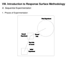
5. Steps of the method The strategy in developing an empirical model through a sequential program of experimentation is as follows: • The simplest polynomial model is fitted to a set of data collected at the points of a first-order design. • If the fitted first-order model is adequate, the information provided by the fitted model is used to locate areas in the experimental region, or outside the experimental region, but within the boundaries of the operability region, where more desirable values of the response are suspected to be.

6. In the new region, the cycle is repeated in that the first-order model is fitted and testing for adequacy of fit. • If nonlinearity in the surface shape is detected through the test for lack of fit of the first-order model, the model is upgraded by adding cross-product terms and / or pure quadratic terms to it. The first-order design islikewise augmented with points to support the fitting of the upgraded model.

7. If curvature of the surface is detected and a fitted second-order model is found to be appropriate, the second-order model is used to map or describe the shape of the surface, through a contour plot, in the experimental region. • If the optimal or most desirable response values are found to be within the boundaries of the experimental region, then locating the best values as well as the settings of the input variables that produce the best response values.

8. 7. Finally, in the region where the most desirable response values are suspected to be found, additional experiments are performed to verify that this is so.

9. B- Illustration of the method with an example For simplicity of presentation we shall assume that there is only one response variable to be studied although in practice there can be several response variables that are under investigation simultaneously.

10. Experience Two controlled Factors Chemical reaction One response Temperature (X1) percent yield Time (X2) An experimenter, interested in determining if an increase in the percent yield is possible by varying the levels of the two factors.

11. Two levels of temperature: 70° and 90°. Two levels of time: 30 sec and 90 sec. Four different design points Four temperature-time settings (factorial combinations) And two repetitions at each point The total number of observations is N = 8

12. Detail The response of interest is the percent yield, which is a measure of the purity of the end product. The process currently operates in a range of percent purity between 55 % and 75 %, but it is felt that a higher percent yield is possible.

14. Representation of the first design

15. First-order model Expressed in terms of the coded variables, the observed percent yield values are modeled as: The remaining term, , represents random error in the yield values. The eight observed percent yield values, when expressed as function of the levels of the coded variables, in matrix notation, are: Y = X  + 

16. Matrix form Vector of error terms Vector of response values Matrix of the design = + Vector of unknown parameters

17. Estimations The estimates of the coefficients in the first-order model are found by solving the normal equations: The estimates are: The fitted first-order model in the coded variables is:

18. ANOVA table – design 1 Test of adequacy

19. Individual tests of parameters To do that the Student-test is used. For the test of: we have And for we have Each of the null hypothesesis rejected at the  = 0.05 level of significance owing to the calculated values, 3.73 and 10.65, being greater in absolute value than the tabled value, T5;0.025 =2.571.

20. Conclusion of the first analysis The first – order model is adequate. That both temperature and time have an effect on percent yield. Since both b1 and b2 are positive, the effects are positive. Thus, by raising either the temperature or time of reaction, this produced a significant increase in percent yield.

21. Second stage of the sequential program At this point, the experimenter quite naturally might ask: If additional experiments can be performed At what settings of temperature and time should the additional experiments be run?” To answer this question, we enter the second stage of our sequential program of experimentation.

22. Contour plots The fitted model: can now be used to map values of the estimated response surface over the experimental region. This response surface is a hyper-plane; their contour plots are lines in the experimental region. The contour lines are drawn by connecting two points (coordinate settings of x1 and x2) in the experimental region that produce the same value of

23. In the figure above are shown the contour lines of the estimated planar surface for percent yield corresponding to values of = 55, 60, 65 and 70 %.

24. Performing experiments along the path of steepest ascent To describe the method of steepest ascent mathematically, we begin by assuming the true response surface can be approximated locally with an equation of a hyper-plane Data are collected from the points of a first-order design and the data are used to calculate the coefficient estimates to obtain the fitted first-order model Estimated response function

25. The next step is to move away from the center of the design, a distance of r units, say, in the direction of the maximum increase in the response. By choosing the center of the design in the coded variable to be denoted by O(0, 0, …, 0), then movement away from the center r units is equivalent to find the values ofwhich maximize subject to the constraint Maximization of the response function is performed by using Lagrange multipliers. Let where  is the Lagrange multiplier.

27. To maximize subject to the above-mentioned constraint, first we set equal to zero the partial derivatives i=1,…,k and Setting the partial derivatives equal to zero produces: i =1,…,k, and The solutions are the values ofxi satisfying or i = 1,…,k, where the value of  is yet to be determined.Thus the proposed next value of xi is directly proportional to the value of bi.

28. Let us the change in Xi be noted by i , and the change in xi be noted by i. The coded variables is obtained by these formulas where (respectively si) is the mean (respectively the standard deviation) of the two levels of Xi . Thus , then or

29. Let us illustrate the procedure with the fitted first-order model: that was fitted early to the percent yield values in our example. To the change in X2, 2=45 sec. corresponds the change in x2, 2=45/30=1.5 units. In the relation , we can substitute i to xi: , thus and 1 = 0.526, so 1=0.526*10=5.3°C .

30. Points along the path of steepest ascent and observed percent yield values at the points

32. Sequence of experimental trials performed in moving to a region of high percent yield values Design two: For this design the coded variables are defined as:

34. The fitted model corresponding to the group of experiments of design two is: The corresponding analysis of variance is: The model is jugged adequate

35. sequence of experimental trials that were performed in the direction two:

37. Retreat to center + 2 iand proceed in direction three

38. Set up design three using points of steps 6, 7, and 8 along with the following two points:

40. Design three was set up using the point at step 7 as its center. It includes steps 6 – 11. If we redefine the coded variables: and then the fitted first-order model is: The corresponding analysis of variance table is:

41. ANOVA table

42. Fitting a second-order model A second-order model in k variables is of the form: The number of terms in the model above is p=(k+1)(k+2)/2; for example, when k=2 then p=6. Let us return to the chemical reaction example of the previous section. To fit a second-order model (k=2), we must perform some additional experiments.

43. Central composite rotatable design Suppose that four additional experiments are performed, one at each of the axial settings (x1,x2): These four design settings along with the four factorial settings: (-1,-1); (-1,1); (1,-1); (1,1) and center point comprise a central composite rotatable design. The percent yield values and the corresponding nine design settings are listed in the table below:

44. Central composite rotatable design

45. Percent yield values at the nine points of a central composite rotatable design

46. The fitted second-order model, in the coded variables, is: The analysis is detailed in this table, using the RSREG procedure in the SAS software:

47. SAS output 1

48. SAS output 2

49. Response surface and the contour plot

50. More explanations • The contours of the response surface, showing above, represent predicted yield values of 95.0 to 96.5 percent in steps of 0.5 percent. • The contours are elliptical and centered at the point (x1; x2)=(- 0.0048; - 0.0857) or (X1; X2)=(135.85°C; 193.02 sec). • The coordinates of the centroid point are called the coordinates of the stationary point. • From the contour plot we see that as one moves away from the stationary point, by increasing or decreasing the values of either temperature or time, the predicted percent yield (response) value decreases.