Download

1 / 68
680 likes | 860 Views
Verified computation with probabilities. This presentation is animated. (Press F5 to display.). Scott Ferson, scott@ramas.com Applied Biomathematics Scientific Computing, Computer Arithmetic and Verified Numerical Computations El Paso, Texas, 3 October 2008. Perspective.

E N D
Verified computation with probabilities This presentation is animated. (Press F5 to display.) Scott Ferson, scott@ramas.com Applied Biomathematics Scientific Computing, Computer Arithmetic and Verified Numerical Computations El Paso, Texas, 3 October 2008
Perspective • Very elementary methods of interval analysis • Low-dimensional, static • Verified computing (but not roundoff error) • Huge uncertainties • Intervals combined with probability theory • Total probabilities (events) • Probability distributions (random variables)
Bounding probability is an old idea • Boole and de Morgan • Chebyshev and Markov • Borel and Fréchet • Kolmogorov and Keynes • Berger and Walley • Williamson and Downs
Terminology • Dependence = stochastic dependence • More general than repeated variables • Independence = stochastic independence • Best possible = tight (almost) • some elements in the set may not be possible
Incertitude • Arises from incomplete knowledge • Incertitude arises from • limited sample size • measurement uncertainty or surrogate data • doubt about the model • Reducible with empirical effort
Variability • Arises from natural stochasticity • Variability arises from • scatter and variation • spatial or temporal fluctuations • manufacturing or genetic differences • Not reducible by empirical effort
They must be treated differently • Variability is randomness Needs probability theory • Incertitude is ignorance Needs interval analysis • Imprecise probabilities can do both at once
Risk assessment applications • Environmental pollution heavy metals, pesticides, PMx, ozone, PCBs, EMF, RF, etc. • Engineered systems traffic safety, bridge design, airplanes, spacecraft, nuclear plants • Financial investments portfolio planning, consultation, instrument evaluation • Occupational hazards manufacturing and factory workers, farm workers, hospital staff • Food safety and consumer product safety benzene in Perrier, E. coli in beef, salmonella in tomato, children’s toys • Ecosystems and biological resources endangered species, fisheries and reserve management $
Total probabilities (events) • Fault or event trees • Logical expressions (Hailperin 1986) • Reliability analyses • Nuclear power plants • Aircraft safety system design • Gene technology release assessments • etc.
Interval arithmetic for probabilities x + y = [x1 + y1, x2 + y2] xy = [x1 y2, x2 y1] xy = [x1 y1, x2 y2] xy = [x1 y2, x2 y1] min(x, y) = [min(x1, y1), min(x2, y2)] max(x, y) = [max(x1, y1), max(x2, y2)] Rules are simpler because intervals confined to [0,1]
Probabilistic logic • Conjunctions (and) • Disjunctions (or) • Negations (not) • Exclusive disjunctions (xor) • Modus ponens (if-then) • etc.
Conjunction (and) P(A |&| B) = P(A) P(B) Example: P(A) = [0.3, 0.5] P(B) = [0.1, 0.2] A and B are independent P(A |&| B) = [0.03, 0.1]
Stochastic dependence Independence Probabilities are areas in the Venn diagrams
Fréchet case P(A & B)=[max(0, P(A) + P(B)–1), min(P(A), P(B))] • Makes no assumption about the dependence • Rigorous (guaranteed to enclose true value) • Best possible (cannot be any tighter)
}certain uncertain Fréchet examples Examples: P(A) = [0.3, 0.5] P(B) = [0.1, 0.2] P(A & B) = [0, 0.2] P(C) = 0.29 P(D) = 0.22 P(C & D) = [0, 0.22]
Switch S1 Relay K2 Relay K1 Timer relay R Motor Pressure switch S From Pump reservoir Pressure tank T Outlet valve Example: pump system What’s the risk the tank ruptures under pumping?
R E5 or K2 E4 K1 or E2 or S1 E1 E3 or and T S Fault tree Boolean expression of “tank rupturing under pressure” E1 Unsure about the probabilities and their dependencies
Results Points, independence Mixed dependencies Fréchet Intervals and Fréchet 105 104 103 Probability of tank rupturing under pumping
Interval probabilities • Allow verified computing of reliabilities • Distinguish two forms of uncertainty • Rigorous bounds always easy to get • Best possible bounds may need mathematical programming because of repeated variables
Typical problems • Sometimes little or even no actual data • Updating is rarely used • Very simple arithmetic calculations • Occasionally, finite element meshes or differential equations • Usually small in number of inputs • Nuclear power plants are the exception • Results are important and often high profile • But the approach is being used ever more widely
Example: pesticides & farmworkers • Total dose is decomposed by pathway • Dermal exposure on hands • Exposures to rest of body • Inhalation (concentration in air, exposure duration, breathing rate, penetration factor, absorption efficiency) • Takes account of related factors • Acres, gallons per acre, mixing time • Body mass, frequency of hand washing, etc.
Worst-case analysis • Traditional method • Mix of deterministic and extreme values • Actually a kind of interval analysis • Says how bad it could it be, but not how unlikely that outcome is
Probabilistic analysis • State-of-the-art method • Usually via Monte Carlo simulation • Requires the full joint distribution • All the distributions for every input variable • All their intervariable dependencies • Often we need to guess about a lot of it
What’s needed • Reliable, conservative assessments of tail risks • Using available information but without forcing analysts to make unjustified assumptions • Neither computationally expensive nor intellectually taxing
Probability bounds analysis • Marries intervals with probability theory • Distinguishes variability and incertitude • Solves many problems in uncertainty analysis • Input distributions unknown • Imperfectly known correlation and dependency • Large measurement error, censoring, small sample sizes • Model uncertainty
Calculations • All standard mathematical operations • Arithmetic operations(+, , ×, ÷, ^, min, max) • Logical operations(and, or, not, if, etc.) • Transformations(exp, ln, sin, tan, abs, sqrt, etc.) • Backcalculation (tolerance solutions)(deconvolutions, updating) • Magnitude comparisons(<, ≤, >, ≥, ) • Other operations(envelope, mixture, etc.) • Faster than Monte Carlo • Guaranteed to bounds answer • Good solutions often easy to compute
Probability box (p-box) Interval bounds on an cumulative distribution function (CDF) 1 Cumulative probability 0 0.0 1.0 2.0 3.0 X
Duality • Bounds on the probability at a value Chance the value will be 15 or less is between 0 and 25% • Bounds on the value at a probability 95th percentile is between 40 and 70 1 Cumulative Probability 0 0 20 40 60 80 X
1 1 0 0 10 20 30 40 10 20 30 Uncertain numbers Probability distribution Probability box Interval 1 Cumulative probability 0 0 10 20 30 40
Probability bounds arithmetic 1 1 A B Cumulative Probability Cumulative Probability 0 0 0 1 2 3 4 5 6 0 2 4 6 8 10 12 14 What’s the sum of A+B?
A+B[4,12] prob=1/9 A+B[5,13] prob=1/9 A+B[7,13] prob=1/9 A+B[8,14] prob=1/9 A+B[9,15] prob=1/9 A+B[9,15] prob=1/9 A+B[10,16] prob=1/9 A+B[11,17] prob=1/9 Cartesian product A = mix(1,[1,3], 1,[2,4], 1, [3,5]) B = mix(1, [2,8], 1, [6,10], 1,[8,12]) A |+| B ~(range=[3,17], mean=[7.3,14], var=[0,22]) A + B ~(range=[3,17], mean=[7.3,14], var=[0,38]) A+B independence A[1,3] p1 = 1/3 A[2,4] p2 = 1/3 A[3,5] p3 = 1/3 B[2,8] q1 = 1/3 A+B[3,11] prob=1/9 B[6,10] q2 = 1/3 B[8,12] q3 = 1/3
A+B under independence 1.00 0.75 0.50 Cumulative probability 0.25 0.00 15 0 3 6 9 12 18 A+B
Generalization of methods • When inputs are distributions, the answers conform with probability theory • When inputs are intervals, it agrees with interval analysis
Where do we get p-boxes? • Assumption • Modeling • Robust Bayes analysis • Constraint propagation • Data with incertitude • Measurement error • Sampling error • Censoring
A tale of two data sets Skinny (n = 6) Puffy (n = 9) 0 0 2 2 4 4 6 6 8 8 10 10 0 0 2 2 4 4 6 6 8 8 10 10 x x
Empirical distributions 1 1 1 Skinny Puffy Cumulative probability Cumulative probability 0 0 0 0 0 2 2 4 4 6 6 8 8 10 10 0 0 2 2 4 4 6 6 8 8 10 10 x x x x
Fitted distributions 1 1 Skinny Puffy Cumulative probability 0 0 0 10 20 0 10 20 x x Statisticians often ignore the incertitude, or treat it as though it were (uniform) variability.
Constraint propagation (lognormal with interval parameters)
Maximum entropy erases uncertainty 1 1 1 mean, std positive, quantile min,max 0 0 0 2 4 6 8 10 -10 0 10 20 0 10 20 30 40 50 1 1 1 min, max, mean sample data, range integral, min,max 0 0 0 2 4 6 8 10 2 4 6 8 10 2 4 6 8 10 1 1 1 (lognormal with interval parameters) min, mean min,max, mean,std p-box 0 0 0 0 10 20 30 40 50 2 4 6 8 10 2 4 6 8 10
Example: PCBs and duck hunters Location: Massachusetts and Connecticut Receptor: Adult human hunters of waterfowl Contaminant: PCBs (polychorinated biphenyls) Exposure route: dietary consumption of contaminated waterfowl Based on the assessment for non-cancer risks from PCB to adult hunters who consume contaminated waterfowl described in Human Health Risk Assessment: GE/Housatonic River Site: Rest of River, Volume IV, DCN: GE-031203-ABMP, April 2003, Weston Solutions (West Chester, Pennsylvania), Avatar Environmental (Exton, Pennsylvania), and Applied Biomathematics (Setauket, New York).
Hazard quotient EF = mmms(1, 52, 5.4, 10) meals per year // exposure frequency, censored data, n = 23 IR = mmms(1.5, 675, 188, 113) grams per meal //poultry ingestion rate from EPA’s EFH C = [7.1, 9.73] mg per kg //exposure point (mean) concentration LOSS = 0 // loss due to cooking AT = 365.25 days per year //averaging time (not just units conversion) BW = mixture(BWfemale, BWmale) // Brainard and Burmaster (1992) BWmale = lognormal(171, 30) pounds // adult male n = 9,983 BWfemale = lognormal(145, 30) pounds // adult female n = 10,339 RfD = 0.00002 mg per kg per day // reference dose considered tolerable HQ = (EF |*| IR |*| C |*| (1|-| LOSS)) |/| (AT |*| BW |*| RfD)
= 1 - CDF Inputs 1 1 Exceedance risk EF IR 0 0 0 10 20 30 40 50 60 0 200 400 600 meals per year grams per meal 1 1 males females C BW 0 0 0 100 200 300 0 10 20 pounds mg per kg
Automatically verified results EF = mmms(1, 52, 5.4, 10) *units('meals per year') // exposure frequency, censored data, n = 23 IR = mmms(1.5, 675, 188, 113) *units('grams per meal') // poultry ingestion rate from EPA’s EFH C = [7.1, 9.73] *units('mg per kg') // exposure point (mean) concentration LOSS = 0 // loss due to cooking AT = 365.25 *units('days per year') // averaging time (not just units conversion) BWmale = lognormal(171, 30) *units('pounds') // adult male n = 9,983 BWfemale = lognormal(145, 30) *units('pounds') // adult female n = 10,339 BW = mixture(BWfemale, BWmale) // Brainard and Burmaster (1992) RfD = 0.00002 *units('mg per kg per day') // reference dose considered tolerable HQ = (EF |*| IR |*| C |*| (1|-| LOSS)) / (AT |*| BW |*| RfD) HQ ~(range=[5.52769,557906], mean=[1726,13844], var=[0,7e+09]) meals grams meal-1 days-1 pounds-1 day HQ = HQ + 0 HQ ~(range=[0.0121865,1229.97], mean=[3.8,30.6], var=[0,34557]) mean(HQ) [ 3.8072899212, 30.520271393] sd(HQ) [ 0, 185.89511004] median(HQ) [ 0.66730580299, 54.338212132] cut(HQ,95%) [ 3.5745830321, 383.33656983] range(HQ) [ 0.012186461038, 1229.9710013] 1 mean [3.8, 31] standard deviation [0, 186] median [0.6, 55] 95th percentile [3.5 , 384] range [0.01, 1230] Exceedance risk 0 0 500 1000 HQ
Uncertainty about distribution shape • PBA propagates uncertainty about distribution shape comprehensively • Neither sensitivity studies nor second-order Monte Carlo can really do this • Maximum entropy hides uncertainty
Dependence • Not all variables are independent • Body size and skin surface area • Common-cause variables • Default risks for mortgages • Known dependencies should be modeled • What can we do when we don’t know them?
Uncertainty about dependence • Sensitivity analyses usually used • Vary correlation coefficient between 1 and +1 • But this underestimates the true uncertainty • Example: suppose X, Y ~ uniform(0,25) but we don’t know the dependence between X and Y