Download
1 / 21
210 likes | 356 Views
Discrete Probabilities. CS5303 – Logical Foundations of Computer Science. Applications of probabilities to CS. Algorithms (average complexity) Probabilistic Algorithms Modeling and Simulation Queuing processes Signal processing. Definition.

E N D
Discrete Probabilities CS5303 – Logical Foundations of Computer Science
Applications of probabilities to CS • Algorithms (average complexity) • Probabilistic Algorithms • Modeling and Simulation • Queuing processes • Signal processing
Definition • Probability: study of processes involving randomness (cards, numbers of phone calls, access to a network, how long is a system survivable etc…) • Probabilities describe the mathematical theory behind random experiments, processes etc…
Trials • Trial/Observation: the result of a random experiment. ωΩ where Ω is the set of all possible results Exercise: what is Ω for • I throw 3 quarters in the air and look at if it’s head or tail • I throw 3 quarters and look at the number of heads • I throw two dice that are distinguishable and look at the combination • Same question with the two dice being indistinguishable
Events • A random event A is a set of results A={ωΩ| A is realized if ω is the result of the experiment} Exercise: in the case where two dice are distinguishable, what is A: the total is at least 10
Relations between events • Certain event Ω • Impossible event • Opposite event Ac • And • Or • Incompatible events A B = • Exhaustive system partition • Implication inclusion AB
Probabilisable space • Definition: TP(Ω) is a σ-algebra if 1. ΩT 2. AT implies AcT 3. nIN, AnT implies nIN AnT • 3. is called σ-additivity • If Ω is finite or countable, we will often take T = P(Ω) (does it satisfy 1,2,3?) • Definition: (Ω,T) is called a probabilisable space
Probability Space • Definition: let (Ω,T) be a prob. Space. Then P:T [0,1] is a probability if: 1. For all A in T P(A) [0,1] 2. P(Ω) = 1 3. If (An)nIN is a family of elements of T disjoint 2 by 2 then P(An) = P(An) • Definition: (Ω,T,P) is a probability space
Exercise • Let Ω be finite, and T = P(Ω). Define P: T[0,1] by P(A) = |A|/|Ω| for A in T. Show that P is a probability.
Properties • P(AB) = P(A)+P(B) – P(AB) • P(Ac) = 1-P(A) • If AB then P(A)P(B) • P(i=1n Ai) i=1nP(Ai) • If An is an increasing sequence for then P(nINAn) = limn P(An) • If An is a decreasing sequence for then P(nINAn) = limn P(An) • P(i=1n Ai) = k=1n(-1)k-1i1<…<ik P(Ai1…Aik) Exercise: A and B shoot a target. A hits 25% and B hits 40%. What is the probability that the target is hit?
Conditional probabilities and independent events • Probability that someone is color blind? • Probability that a man a color blind? • Probability that a woman is color blind? • Definition: Let (Ω,T,P) be a probability space and A a non-null event then P(B|A) = P(AB)/P(A) • Property: P(.|A) is a probability over (Ω,T)
Example • Consider families with 2 children. Then Ω={BB,GG,BG,GB} writing the children in decreasing order w.r.t age. Knowing there is at least one boy, what is the probability that there are 2? • A={BB,GB,BG}, B={BB} • P(A|B) = |AB|/|A| = 1/3
Generalization • Property: Let A1,…,An be events • P(A1…An)=P(A1)P(A2|A1)P(A3|A1A2)… P(An|A1…An-1) Proof is by induction on n Exercise: consider the transmission of a message yes or no in a given population. Each person transmits the message received with probability p and the opposite message with probability q=1-p. Let Xn be the msg received by the nth individual In. We assume that I0 gives yes to I1. What is P(In received yes)?
Bayes Formula • Lemma: Let (Ω,T,P) be a probability space and (Ak)kIN an exhaustive system, then if B is an event: P(B)=kIN P(B|Ak)P(Ak) Exercise: prove it • Theorem: if B is not null then under the hypotheses of the lemma: P(An|B)=P(An)P(B|An)/kIN P(B|Ak)P(Ak)
Application • A city is divided in 3 political areas Area number % of electors score of C • 30 40 • 50 48 • 20 60 An elector is picked at random. What is the probability he/she voted for C? Given that e has voted for C, what is the probability that e is from area 3?
Random Variables • Definition: Let (Ω,T,P) be a probability space. A (real valued) random variable on this space is a function X:ΩIR such that for any open interval I of IR, X-1(I)T • Under the same definition, a discrete random variable from Ω to D is such that X-1(d) T for any d in D
Distribution • Definition: let X be a d.r.v. The probability distribution of X is defined by PX(d) = P(X=d) • The repartition function of X is defined by FX(d) = P(X<d) = d’<dPX(d’)
Mathematical Expectation • Definition: if X is a d.r.v then its mathematical expectation is defined by E(X) = ωΩ X(ω)P(ω)=dD d.P(X=d) • The mathematical expectation is a linear form over the space of discrete random variables (defined on the same sets) • Property: if Y=f(X) with f:DIR, then E(Y) = dD f(d).P(X=d)
Variance - Covariance • The quadratic moment (when it exists) is defined by E(X2) = dD d2.P(X=d) • The variance is defined by var(X) = E(X2)-(E(X))2 • The covariance of X,Y is defined by Γ(X,Y)=E(X-E(X))E(Y-E(Y))=E(XY)-E(X)E(Y) • The coefficient of correlation is defined by ρ(X,Y)= Γ(X,Y)/σ(X)σ(Y)
Properties • If X and Y are independent random variables then • E(XY)=E(X)E(Y) • var(X+Y) = var(X)+var(Y)
Classical distributions • Bernoulli law: X:{0,1}{0,1}. Law is denoted by B(p). P(X=1)=p, P(X=0)=1-p • Find E(X) and var(X) • Binomial law: some of n independent Bernoulli law denoted b(n,p) • Find E(X) and var(X) • Law of Poisson: X:ΩIN follows a law of poisson of parameter λ if P(X=k) = e-λ.λk/k! • Find E(X) and var(X) • For n large and p small, the law of Poisson is an approximation of the binomial law