Download
1 / 31
310 likes | 318 Views
Introduction to Regression Analysis. March 21-22, 2000. Review of correlation. Correlation examines the relationship between two variables. The relationship can be expressed as a graph called a scattergram. Correlation. Correlation.

E N D
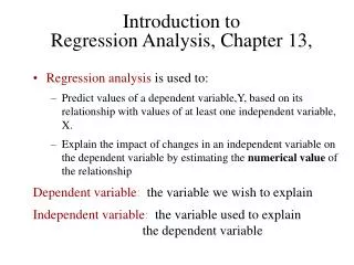
Introduction to Regression Analysis March 21-22, 2000
Review of correlation • Correlation examines the relationship between two variables. • The relationship can be expressed as a graph called a scattergram.
Correlation • The relationship between the two variables can also be expressed as a number called the correlation coefficient. • The values of correlation coefficients range from -1 to +1. • The most commonly used measure of correlation is the Pearson product-moment correlation coefficient, designated as “r”.
Correlation • A positive correlation indicates that high values of one variable correspond with high values of the other variable and low values correspond with low values. When this occurs, the r value is a positive number (r=.66) • A negative correlation indicates that when the value for one variable is high the value for the other variable will be low. When this occurs, the r value is a negative number (r=-.66)
Correlation • A correlation coefficient of -1 or +1 represents a perfect correlation. • r = -1 is a perfect negative relationship • r = +1 is a perfect positive relationship • A correlation of 0 (r = 0) means that no linear relationship exists between the two variables. • The stronger the relationship between the two variables, the closer r is to 1.
Correlation • r = 0.82 • There is a strong positive relationship. As female literacy increases in a country, female life expectancy also increases.
Correlation • R = - 0.84 • There is a strong negative relationship. As female literacy in a country increases, infant mortality decreases.
Correlation • r = 0.37 • There is a moderate, positive relationship between birth rate and death rate for a country.
Correlation • Web site: Guessing correlations
Review of t test • The t test is an inferential statistic that compares the means of two different groups. • It asks the question, “are the differences between the two groups statistically significant or did the differences occur randomly (by chance)?”
Review of t test • Steps in hypothesis testing • formulate a research and null hypothesis • select an alpha level • calculate a test statistic (in this case “t”) • compare observed to critical value • Rule of thumb for t • The critical value of t for a two-tailed test with = .05 and n>30 is 2.04 • If these criteria are met, a t value that exceeds 2 is statistically significant.
Review of t test • In research articles, the t value is usually reported as being statistically significant or not by indicating p values. • p <.05 means the t value is statistically significant at an alpha level of .05. In other words, you are 95% confident. • Other commonly used levels of statistical significance include • p <.01 • p <.001
Review of t test • By custom, * is also used to indicate statistical significance. • p <.05 * • p <.01 ** • p <.001 ***
Review of t test • Statistical significance essentially means “difference.” It also means that the difference is large enough to assume that it did not occur by chance. • It does not mean that the finding, however, is important. That requires theory and other types of evidence.
Regression Analysis - Introduction • Often, researchers are interested in examining the relationships between two or more variables. • Contingency tables can do this when we have nominal or ordinal level data and not too many categories. • When we have interval level data, we can use another statistical technique called regression analysis. • Model testing
Regression Analysis - Introduction • Regression analysis is one of the strongest statistical tools we have in the social sciences. It takes full advantage of the information we have in our data. • Measure associations among variables • infer population characteristics based on a sample • argue, by statistically manipulating variables, causal links between variables • forecast outcomes
Regression Analysis - Introduction • Suppose we are looking at the relationship between two variables: weight of a package of apples and price. If the scale is accurate, it looks like this.
This line, or relationship, can be displayed as a mathematical formula also. • Y = .79X • Where Y is the price of the bag of apples, and X is the weight of apples. • .79 is the price per pound • There is a positive perfect relationship between the two variables. r= 1.0
r= .96 • Suppose the scale was a little off. Now the line might look like this. 12 10 8 6 4 2 WEIGHT 0 0 20 40 60 80 100 120 140 PRICE
Now there is not a perfect relationship between the two variables, so it can not be expressed as a single equation. • We can, however, estimate a line that is the “best fit” of the data. This is one of the things that regression analysis does.
Bivariate Regression Analysis • We will begin with a two-variable model. • A regression model can best be expressed as an equation.
a = the constant or Y intercept • b = the regression coefficient or slope • Y = the predicted value of Y, the dependent variable • X = the independent variable
a = the constant or Y intercept • This is what Y would equal if X = 0. • X represents the possible values of the independent variable. • = the slope of the line. The slope is the change in Y per unit change in X. As slope approaches 0, it indicates that there is no relationship.
Y (DV) is crime rate (per 100,000) • X (IV) is unemployment (in %) • For example, if = 120, then the slope tells us that for every one percent increase in unemployment, the crime rate will go up 120 per 100,000 persons.
Regression gives us a line that is the “best fit” of the data. Because the relationship between the variables is not perfect, all the points will not fall exactly on the line. OVERHEAD • Therefore we refer to Y as the predicted value of Y also called Y hat. • The difference between the actual Y and the predicted Y is referred to as the residual.
OVERHEAD • Scatterplot and regression line of car repair costs and miles
Correlation coefficient • One of the major uses of regression analysis is to estimate population characteristics. The regression line is the best estimator of the linear model. If any other line were placed on the scatterplot, the sum of the square residuals (distance between Y and predicted Y) would be larger.
Correlation coefficient • A test of goodness of fit lets us determine how well our equation fits the data. • One way to assess this is visually. • A second way is the correlation coefficient. (Pearson’s r).
Correlation coefficient • Another test is the coefficient of determination referred to as r2. • r2 indicates the proportion of the variance in the dep var associated with or explained by the indep var(s). • In our previous car repair costs example, the r2 = .87 indicating that 87% of the variance in car repair costs is explained by mileage.
Correlation coefficient • When is r2 big enough? It depends.