Download

1 / 12
280 likes | 704 Views
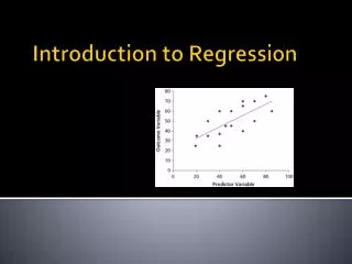
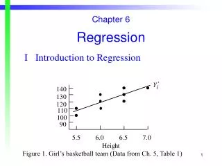
Basic Introduction to Regression. Linear Regression. When the scores on one variable (X) are used to predict the scores on another variable (Y), the scores for each participant on both variables (X, Y) are plotted on a graph called a scatterplot.

E N D
Linear Regression • When the scores on one variable (X) are used to predict the scores on another variable (Y), the scores for each participant on both variables (X, Y) are plotted on a graph called a scatterplot. • Typically, the DV is denoted as the Y variable, and the IV is denoted as the X variable. • Needless to say, when making inferences based upon the value of one variable (e.g., GRE score) to predict the scores on another variable (e.g., graduate school GPA), there is going to be some amount of error. • The problem that is dealt with in regression is to find the “best” fitting regression line where the errors are minimized. • The technique for finding the best-fitting straight line for the dataset is called regression.
Basic Points… • The best-fitting line is the one that is closest to the data points • We want the errors in predicting Y to be as small as possible • There is always one, and only one, line that minimizes the error
Regression Equation • The equation used to estimate (predict) any Y point from a given X point is as follows: Y = b(X) + a Whereby Y = A participant’s score on Y X = A participant’s score on X b = Regression coefficient a = The Y-intercept (value of Y when X=0)
Regression Coefficient • The slope, or steepness, of this line is called the regression coefficient. • Hence, regression coefficient = slope • The regression coefficient is also called a beta weight • The formula for the regression coefficient is as follows: b = rxy * (S Y) (S X) Whereby b = slope (beta weight) r = Pearson correlation Sx = Standard deviation of X Sy = Standard deviation of Y
Regression Intercept • Remember that X and Y represent different but related variables. Therefore, Y has a particular value when there is no value for X. • The value of Y when X=0 is called the regression intercept. • The formula for the regression intercept is as follows: a = MY – (b * MX) Whereby a = regression intercept b = regression slope My = Mean of Y Mx = Mean of X This formula represents the point at which the regression line crosses the Y axis.
Predicting Y from X • Once the regression coefficient and the regression intercept have been found, the corresponding values can be used to predict what value any given individual will have on the DV (y), given a particular score on the IV (x). • Given the regression equation, a score for Y can be plotted on a graph for every corresponding score on the graph – the line drawn through these scores is the regression line, and is the best estimate of Y from X. • How much did we increase the predictability of Y by using regression? Calculate R2
Using the example from yesterday…. • The ACT math and science scores (respectively) for 8 students are shown below. Compute the regression equation for Y (science ACT scores). Use the equation to predict a science ACT score for a student scoring 33 on the math ACT. • Student 1: 26, 24 • Student 2: 22, 24 • Student 3: 13, 10 • Student 4: 30, 31 • Student 5: 12, 17 • Student 6: 15, 15 • Student 7: 19, 21 • Student 8: 20, 16
Introduction to Multiple Regression • Multiple regression is used when there is one Y criterion variable and 2 (or more) X predictor variables. • For example, we might be interested in predicting graduate school success with both GRE score and undergraduate GPA.
The Regression Equation with 2 Predictors • Y = b1X1 + b2X2 + a Whereby Y = A participant’s score on Y X1 = A participant’s score on X1 X2 = A participant’s score on X2 b1 = Regression coefficient for X1 b2 = Regression coefficient for X2 a = The Y-intercept
More on regression weights…. • b1 provides the answer to the question: Suppose I already have X2 in my prediction equation. Given that X2 is in the equation, is it worthwhile to assign some weight to X1? In other words, does X1 help predict Y over and above X2? The answer is that if b1 is significantly different than 0, then X1 helps predict Y over and above the use of just X2. • Or, a unit change in X1 is predicted to make a b1 change in Y, assuming X2 is held constant.
Multiple R2 • How much did we increase the predictability of Y by using regression? Calculate Multiple R2 (the squared multiple correlation) • There is no single unambiguous way to answer the question of how much of the squared multiple correlation is due to X1 and how much is due to X2 • Use Venn Diagram example