Download
1 / 15
150 likes | 325 Views
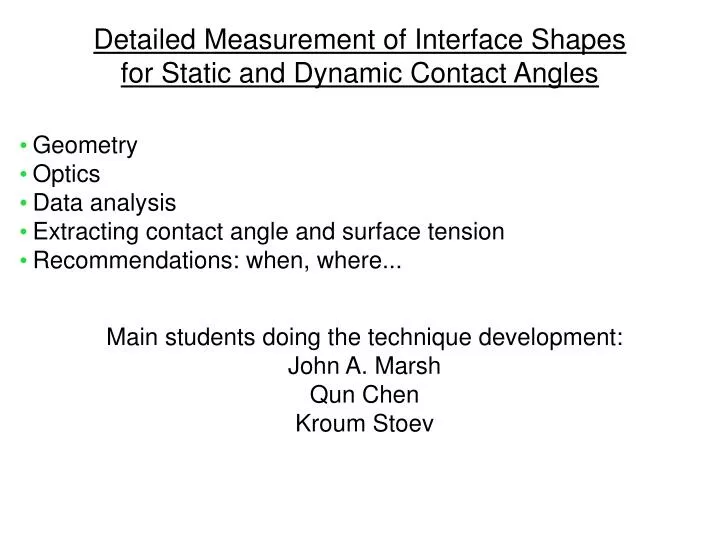
Detailed Measurement of Interface Shapes for Static and Dynamic Contact Angles. Geometry Optics Data analysis Extracting contact angle and surface tension Recommendations: when, where. Main students doing the technique development: John A. Marsh Qun Chen Kroum Stoev. Geometry. D T.

E N D
Detailed Measurement of Interface Shapes for Static and Dynamic Contact Angles • Geometry • Optics • Data analysis • Extracting contact angle and surface tension • Recommendations: when, where... Main students doing the technique development: John A. Marsh Qun Chen Kroum Stoev
Geometry DT Highest point on line of sight Cap Length • Tube Diameter: DT = 2.5 cm • DT >> Cap Length (1.5 mm): • Azimuthal curvature small effect on shape and flow • Easy to focus, sharp meniscus seen on meridian plane(unlike flat plate) • Unlike spreading drop, outer length scale very large • Cylinder: No "end effects"
Optics: Kohler Illumination Condenser Focal plane • Image of light source forms at condenser aperture
Optics: Kohler Illumination • Image of source aperture forms at object plane • Condenser aperture: controls cone angle • Source aperture: controls illuminated spot size • Uniform illumination key to making physical edge parallel to equi-intensity contour Result: uniformly illuminated, in-focus image of source aperture
Image Quality Highest curvature in line of sight: Sharpest Image • Uniformly flat surface: • Lowest curvature along line of sight • Fuzzier image • 80° ≤ Contact angles ≤ 100°: Can’t measure because contact line hidden • Usually meniscus edge sharp out to >1.4 mm
Image Quality - 2 • Interfaces meeting at the contact line: • Diffraction patterns interfere& cause distortion • Contact angle < 5°: • No problem • Can get interface all the way through contact line • Larger contact angles: • Safely down to 15µm to 20µm from contact line • Best conditions can get closer
Menisci in Depression • Can be measured • Light path through liquid • PIV possible • Edge finder output: interface slope vs. position • Slope: One derivative closer to curvature than x-y data • Question: do "equal intensity levels" follow physical edge? • A: Calibration
Calibration • Needed due to small distortions near edges • Mechanical shapes (e.g., straight edge) not good enough • How straight is the edge? • Use static capillary shape: • Known exact theoretical form: Young-Laplace Eq. • Use Static Contact Angle and Surface Tension as fitting parameter • Two-parameter fit: contact angle & surface tension uncoupled • Difference (Data-Fit): • No systematic deviation from zero • Strict criterion imposed – cloud of data does not move more than 1/3 width off zero line
Fitting Details • Fitting AWAY from contact line crucial • Why • All surfaces have contact angle hysteresis • With hysteresis comes contact line brokenness • ...which leads to interface shape fluctuations • Fluctuations die out: scale larger than contact line waviness! • Need to fit beyond folding to get “contact angle” & surface tension • Global contact angle: boundary condition for meniscus beyond folds
Analysis • We fit theoretical models to the interface data • Young-Laplace (static theory) • Cox-Dussan composite asymptotics (Newtonian, viscous theory) • Extract: • Static contact angle & surface tension from fit to Young-Laplace • "Dynamic" apparent contact angle from fit to Cox-Dussan • Requirements • (Best fit - Exptal data) free of systematic deviation
Accuracy • Data cloud ~2° thick (but ~1° RMS) • Contact angle accuracy ~1°or less • Mostly Run-to-Run variation • Good accuracy due to calibration with static shape • High precision in local interface angle from fitting to large number of data points to determine one interface angle • Very accurate (~0.25deg) measurement of interface shape
Recommendations • Kohler illumination less important than uniform illumination • Good resolution from 15µm to 1500µm from contact line • Perhaps not strictly necessary for static unless detailed shape needed (i.e., could use "2-point" for statics...) • Necessary when detailed interface shapes needed • Necessary for dynamic contact angle
Optics: Kohler Illumination • Settings: • Source aperture: just large enough to illuminate entire field of view • Larger condenser aperture: more fuzzy, less contrast, more depth of focus • Smaller condenser aperture: more contrast, more diffraction fringing around contact line • Cylindrical geometry requires not-too-large depth of focus Result: uniformly illuminated, in-focus image of source aperture