Download
1 / 18
190 likes | 322 Views
Monitoring the Ocean State from the Observations. Stéphanie Guinehut Sandrine Mulet Marie-Hélène Rio Gilles Larnicol Anne-Lise Dhomps. Introduction. Our approach : Consists of estimating 3D-thermohaline and current fields using ONLY observations and statistical methods

E N D
Monitoring the Ocean State from the Observations Stéphanie Guinehut Sandrine Mulet Marie-Hélène Rio Gilles Larnicol Anne-Lise Dhomps
Introduction • Our approach : • Consists of estimating 3D-thermohaline and current fields using ONLY observations and statistical methods • Represents a complementary approach to the one developed by forecasting centers – based on model/assimilation techniques • “Observation based” component of the Global MyOcean Monitoring and Forecasting Center lead by Mercator Océan • Previous studies have shown the capability of such approaches : • In producing reliable ocean state estimates (Guinehut et al., 2004; Larnicol et al., 2006) • In analyzing the contribution and complementarities of the different observing systems (in-situ vs. remote-sensing) (2nd GODAE OSE Workshop, 2009)
The principle The observations The method The products Global 3D Ocean State [T,S,U,V,H] Weekly – 1993-2009 [0-1500m] 24 levels [1/3°] MyOcean V1 RT/RAN Altimeter, SST, winds Guinehut et al., 2004 Guinehut et al., 2006 Larnicol et al., 2006 Rio et al., 2011 + MDT estimate Intercomparison with independent data sets and model simulations Analysis of the ocean variability Observing System Evaluation T/S profiles, surface drifters
Global T/S Armor3D - Method vertical projection of satellite data (SLA, SST) combination of synthetic and in-situ profiles 1 T(x,y,z,t) = (x,y,z,t).SLAsteric + (x,y,z,t).SST’ + Tclim (x,y,z,t) S(x,y,z,t)=’(x,y,z,t).SLAsteric + Sclim (x,y,z,t) 2 synthetic T(z), S(z) SLA, SST multiple linear regression 1 optimal interpolation 2 in-situ T(z), S(z) Armor3D T(z), S(z)
Armor3D - 1993-2009 reanalysis NCEP Reynolds OI-SST 1/4° daily - 04/07/2007 SSALTO-DUACS MSLA 1/3° weekly DT - 04/07/2007 Synthetic T’ – at 100m Arivo climatology – July – T at 100 m
Armor3D - 1993-2009 reanalysis In-situ observations – Coriolis data center Synthetic T’ – at 100m Armor3D T’ Argo T’
Armor3D - Hydrographic variability patterns • Temperature variability over the 2004-2008 period (global zonal averaged) : Synthetic SODA 2.2.4 ARMOR3D SCRIPPS • Very similar results for Synthetic/ARMOR3D/SCRIPPS • No bias introduced by the method • Very promising to study the variability of the 1993-2000 period which suffers from poor in-situ measurements coverage 2008 2004 2005 2006 2007
Hydrographic variability patterns • Temperature variability from 1993 to 2008 (global zonal averaged) : 2001 2005 1993 1997 2008
Armor3D - Hydrographic variability patterns • Salinity variability over the 2004-2008 period (global zonal averaged) : SODA 2.2.4 Synthetic SCRIPPS ARMOR3D 2004 2005 2006 2007 • Argo obs sys mandatory 2008
Global U/V/H Surcouf3D - Method Surcouf : Field of absolute geostrophic surface currents weekly - 1/3° Armor3D : 3D T/S fields weekly - 1/3° - [0-1500]m Surcouf3D 3D geostrophic current fields weekly (1993-2008) 1/3° - 24 levels from 0 to1500m
Surcouf3D - Comparison with model outputs • Vertical section at 60°W, in 2006 *geost. current with level of no motion at 1500m Armor3D* Surcouf3D at 500m Surcouf3D GLORYS at 500m GLORYS
Surcouf3D - Validation of 1000-m currents • Global statistics over the Atlantic outside the equateur (10°S-10°N) • Comparison between 3 different methods (Surcouf3D, GLORYS, Armor3D) and in-situ observations (ANDRO) at 1000 m over the 2006/2007 period (Taylor, 2001) Meridionalcomponent ● SURCOUF3D (weekly, 1/3°) ▲GLORYS = Mercator-Ocean reanalysis (weekly, 1/4°) Ferry et al., 2010 ♦ Armor3D= geostrophic current with level of no-motion at 1500m (weekly, 1/3°) ● ANDRO = 1000-m currents from drifting velocities from the Argo floats (≈10days, ≈50/100km) Ollitraut et al, 2010 skill score • Results are very similar for the zonal component Correlation coefficient Standard deviation (cm/s) Standard deviation (cm/s)
Surcouf3D - Validation Meridionalvelocities (cm/s) Zonal velocities (cm/s) • Comparison with GoodHope VM-ADCP observations from 14/02–17/03/2008 ADCP obs courtesy of S. Speich SURCOUF3D ADCP • Good correlation with independent in-situ obs. • Other time series to be compared 14/02/08 17/03/2008
Surcouf3D - Validation • Comparison with RAPID current-meters in the Western boundary current off the Bahamas from April 2004 to April 2005 Florida Africa 26.5°North 76.5°West SURCOUF3D RAPID (current meters) GLORYS • Good correlation with independent obs., and with GLORYS • Importance of in-situ T/S profiles obs at depth for the inversion of the current
Surcouf3D - AMOC variability at 25°N • Comparison with Bryden et al, 2005(section at 24.5° from Africa to 73°W and at 26.5°N off Bahamas) Floride Strait Transport from electrical cable (Bryden et al,2005) AMOC= Geost + Ekman + Florida (Surcouf3D, Bryden et al., 2005) Ekman Transport from wind stress ERAInterim Geostrophic Transport from 75°W to 15°W and from the surface to 1000m (Surcouf3D,Bryden et al., 2005) • Very consistent with Bryden et al, 2005 • Hight inter-annual variability • Hard to distinguish a long-term trend
Surcouf3D - AMOC variability at 26.5°N • Comparison with RAPID and GLORYSfrom April 2004 to December 2007 • (monthly means + 12-month filtered) • Similar seasonal cycle • Amplitude differences ~ 10% • Higher variability in Surcouf than in Glorys that has to be further analyzed SURCOUF3D RAPID GLORYS
Conclusions / Perspectives • Armor3D/Surcouf3D tools are very useful : • to perform intercomparison exercices • to study the interannual variability of the hydrographic patterns, the AMOC … • Intercomparison studies will be continued between Armor3D and Surcouf3D and MyOcean global reanalysis • Further study the ocean state (T/S variability, MOC, Heat/Salt transport) in key regions and for the 1993-2009 periods • Armor3D/Surcouf3D reanalysis are distributed as part of MyOcean
… • …