Download
1 / 49
500 likes | 579 Views
Cost Behavior. Chapter 6. Objective 1. Identify key features of various cost behaviors. Cost Behavior. How costs change in response to changes in volume Variable costs Fixed costs Mixed costs. Variable Costs. Change in total in direct proportion to changes in volume

E N D
Cost Behavior Chapter 6
Objective 1 Identify key features of various cost behaviors
Cost Behavior • How costs change in response to changes in volume • Variable costs • Fixed costs • Mixed costs
Variable Costs • Change in total in direct proportion to changes in volume • Total variable costs = variable cost per unit of activity x volume of activity
Fixed Costs • Do not change over wide ranges of volume
Mixed Costs • Contain both variable and fixed components
Mixed Costs Variable Fixed
S6-1 F ____ a. Depreciation on equipment used to cut wood enclosures ____ b. Wood for speaker enclosures ____ c. Patents on crossover relays (internal components) ____ d. Crossover relays ____ e. Grill cloth ____ f. Glue ____ g. Quality inspector’s salary V F V V V F
Objective 2 Forecast costs using cost equations
Cost Equation Total costs = Total variable costs + Total fixed costs y = vx + f y = total cost v = variable cost per unit of activity (slope) x = volume of activity (x) f = fixed cost over a given period of time (vertical y intercept)
Relevant Range • Band of volume where total fixed costs remain constant and variable cost per unit remains constant. • Outside the relevant range, the cost either increases or decreases
Other Cost Behaviors Step costs – fixed over small range of activity, then jump to new fixed level
Other Cost Behaviors Curvilinear Costs
E6-17 1. Variable costs per unit: $2,625 / 3,500 garments = $0.75 Total fixed costs: $2 x 3,500 garments = $7,000
7,000 $1,500 7,000 $2,625 7,000 $3,750 $8,500 $9,625 $10,750 E6-17 1.
E6-17 3. Actual costs at 2,000 garments $8,500 Total predicted costs: ($2.15 × 2,000 garments) (4,300 ) Underestimated costs $4,200
E6-18 a. 1,000 x $26.43 $26,430 b. Total costs $26,430 Less total fixed costs (18,000) Total variable costs $8,430 ÷ 1,000 Variable cost per mailbox $8.43
E6-18 c. y = $8.43x + $18,000 d. $26.43 x 1,200 mailboxes $31,716 e. y = ($8.43 • 1,200) + $18,000 = $28,116
E6-18 f. Using average at 1,000 $31,716 Using cost equation 28,116 $3,600
Objective 3 Determine cost behavior using account analysis, the high-low method, and regression analysis
High-Low Method • Method to separate mixed costs into variable and fixed components • Select the highest level and the lowest level of activity over a period of time
High-Low Method – E6-21 Step 1: Find slope of the mixed cost line (variable cost/unit) = Δ in cost (y) / Δ in volume (x) ($5,748-$5,020) ÷ (17,300-14,500) $728 ÷ 2,800 = $0.26
High-Low Method – E6-21 Step 2: Find the vertical intercept (fixed costs) = Total mixed cost – Total variable cost $5,748 – ($0.26 • 17,300) = $1,250 or $5,020 – ($0.26 • 14,500) = $1,250
High-Low Method – E6-21 Step 3: Create and use an equation to show the behavior of a mixed cost Y = $0.26 per mile + $1,250 Predicted operating costs at 15,000 miles: ($0.26 • 15,000) + $1,250 = $5,150
Regression Analysis • Statistical procedure to find the line that best fits data • Uses all data points • Results in equation of line and an R-square value
R-Square Value • “Goodness of fit” • How well does the line fit the data points? • Ranges from 0 to 1 • “0” – no relationship between costs and volume – activity is not a cost driver • “1” – perfect relationship – activity is a cost driver
Data Concerns • Seasonal variations • Inflation • Outliers – abnormal data points
E6-22 5. y = 0.29x + 802.39 y = ($0.29 • 15,000) + $802.39 y = $5,152.39
Objective 4 Prepare contribution margin income statements for service firms and merchandising firms
Traditional Income Statement Sales - Cost of Goods Sold Gross Margin - Selling,general & administrative costs Operating Income
Contribution Margin Income Statement Sales - Variable Costs Contribution Margin - Fixed Costs Operating Income
Contribution Margin Income Statement • Predict how changes in volume will affect operating income
E6-25 Rachel’s Rock Shop Income Statement For the year ending 20XX Revenue: Sales Revenue (27,000 + 7,000) $34,000 Rental Revenue 22,000 Lesson Revenue 40,000 Total Revenue $96,000 Less: Cost of Goods Sold (7,500 + 2,000) (9,500) Gross Margin $86,500 Less Operating Costs: Depreciation $ 4,000 Employee Salary expenses 30,000 Musician wages 25,000 Lease 12,000 Total operating costs 71,000 Operating Income $15,500
E6-25 Rachel’s Rock Shop Contribution Margin Income Statement For the year ending 20XX Revenue: Sales Revenue (27,000 + 7,000) $34,000 Rental Revenue 22,000 Lesson Revenue 40,000 Total Revenue $96,000 Less: Variable Costs Cost of Goods Sold (7,500 + 2,000) $ 9,500 Musician wages 25,000 Total Variable costs (34,500) Contribution Margin $61,500 Less Fixed Costs: Depreciation $ 4,000 Employee Salary expenses 30,000 Lease 12,000 Total fixed costs (46,000) Operating Income $15,500
Objective 5 Use variable costing to prepare contribution margin income statements for manufacturers (Appendix)
Variable Costing • Assigns only variable manufacturing costs to products • Direct materials • Direct labor • Variable manufacturing overhead • Fixed manufacturing overhead = period cost • Contribution margin income statements • For internal management decisions
Absorption Costing • Required by GAAP for external reporting • Assign all manufacturing costs to product • Direct materials • Direct labor • Variable manufacturing overhead • Fixed manufacturing overhead • Traditional income statement
E6-26 * computation of variable cost of goods sold
E6-26 Incremental analysis: Increase in contribution margin(($35-20) x 15,000 goggles) $225,000 Increase in fixed costs (150,000) Increase in operating income $75,000