Download
1 / 43
430 likes | 559 Views
Learning Issues in Drug Discovery. Joe Verducci Ohio State University Snowbird, June 2003. The Basic Learning Problem. Given a training set of biologically active and inactive chemical compounds, develop a classification rule based on the structural features of the compounds.

E N D
Learning Issues in Drug Discovery Joe Verducci Ohio State University Snowbird, June 2003
The Basic Learning Problem • Given a training set of biologically active and inactive chemical compounds, develop a classification rule based on the structural features of the compounds. • Activity is determined from bioassays; for example, it might be the ability of a compound to inhibit the growth of a specific type of cancer cell. • Structural features are coded as (long—up to lengths of 30K) binary strings, indicating the presence of basic molecular descriptors.
Examples of Molecular Descriptors Benzenes Heterocycles Functional Groups Pharmacophores Spacer groups
Outline of Issues • How to choose an appropriate kernel? • Biological heuristics • Localization: use class membership in constructing kernels • Identifying groups of similarly structured active compounds • Recursive Partitioning • Simulated Annealing • Clustering chemical classes • COSA • Jaccard/Tanimoto metric • Relationships between features • Over different types of activity • Information from relational databases • Feature assembly • How to choose molecules for the training set?
“Key” to receptors comprises up to 3 features. There may be several receptors. Features around a “key” may prevent its use. Physical properties of a compound may inhibit its approach to the receptor. Suggests weighted polynomial kernel. Suggests non-zero weights over several groupings of features. Gives interpretation to negative weights Suggests that simple weightings apply only to similar types (“local” classes) of compounds. Biological Heuristics
Discovery Goals beyond Classification • Weightings should be interpretable (concentrated on only a few feature-combinations). • If we know what features make a members of a class of compounds active for one type of cell (cancer) and which features make members of this class inactive against another type (normal), it may be possible to design a new drug in that class with both sets of features. • Understand how kernels adapt to classes
Localization • Structural Activity Relationship (SAR) • about a 50 year history in Chemistry • all analyses done using a small group of similar compounds • most analyses done with continuous variables (e.g. lipophilicity, BCUTS) • SVM methods now enable analyses with many binary variables • How to identify relevant “small groups” from a large database? • Concentrate on pockets of active compounds • Concentrate on “natural” chemical classes
Clustering active groups • Recursive Partitioning (RP) • Split database sequentially according to the feature that maximizes difference in mean activity and/or proportion of actives • RP + Simulated Annealing (RPSA) • Stochastic search for combinations of features that approximately optimize split
Ave pGI50 = 4.47 Freq = 28,297 Ave pGI50 = 4.44 Freq = 27,521 Ave pGI50 = 5.36 Freq = 776 Ave pGI50 = 4.4 Freq = 25,408 Ave pGI50 = 4.92 Freq = 2,113 Ave pGI50 = 5.17 Freq = 700 Ave pGI50 = 7.08 Freq = 76 Recursive Partitioning (RP) Applied to LNS-H23 activity in NCI database
Legend (Ave. pGI50) > 7 6 – 7 5 – 6 < 5 RP Tree 0 82 1 83 94 2 93 84 42 3 85 92 43 44 4 27 91 86 22 5 39 28 87 90 45 23 26 21 36 29 40 41 88 89 6 61 46 24 25 37 38 30 35 62 71 14 7 56 47 31 32 70 72 79 63 18 15 11 8 57 60 48 55 33 34 73 74 80 81 64 67 19 20 16 17 12 13 10 58 59 54 49 9 75 78 65 66 68 69 50 53 76 77 51 52 RP parameters: max p-value = 0.01, min set size = 50
Recursive Partitioning (RP) Advantages • Useful for explaining complex, nonlinear response. • Handle very large descriptor sets with continuous, discrete, or categorical variables • Handle very large data sets Disadvantages • Only optimizes one variable at a time • Looks at few combinations of descriptors • Most terminal nodes involve many negative descriptors
Stochastic Tree Search • At each node, simulated annealing is used to find a combination of structural features • Control parameters: • Number of features (descriptors) • Minimum node size • Maximum negative features • Number of tree levels • Want to find local optima • Modification -- drop certain features in the process
0 1 (1) Legend (Ave. pGI50) > 7 6 – 7 5 – 6 < 5 (2) 2 3 (3) (4) 4 5 (5) (6) 6 7 (7) (8) 8 (9) 9 (10) 10 Stochastic Tree Node Ave.pGI50 Count Features 1 7.35 51 oxetane, 3-oxy-; hdonor-path8-hdonor 2 7.49 54 benzene, 1-carbonyl, 4-(2-oxyethyl);hdonor-path8-pcharge 3 7.11 53 carbonyl, oxymethyl-; pyridine, 2-(alkenyl, cyc)- 4 6.66 52 oxepin, 3-oxymethyl-; alcohol, s-alkyl- 5 7.6 60 benzene, 1,3-dimethoxy-; cycloheptatriene, 1,3,5- RP/SA parameters: min set size = 50, number of features in combination = 2.
0.0 0.2 0.4 0.6 0.8 1.0 Clustering Active Compounds
Active Outliers (n-Bu)3PbCl 0.0 0.2 0.4 0.6 0.8 1.0
Clustering Easily Identified Chemical Classes • Jaccard/Tanimoto metric • Most related to activity (Near Neighbor rules comparing metrics -- Peter Willett) • Discounts similarity based on common absence of structures • Previous clustering just used active compounds. Now use all compounds. This is needed to see if test compound is close to an inactive class. • COSA • Friedman and Meulman (2002) • Weighs different features by (estimated) class to determine distances between objects in the same (estimated) class • Results not yet ready.
Tanimoto Coefficient c = # bits on in both A and B a = # bits on in A b = # bits on in B d = # bits off in both A and B Tanimoto Coefficient Tanimoto Coefficient Complement Measures similarity using on bits Measures similarity using off bits
R-Group Analysis ofColchicine Class 38 compounds Ave pGI50 = 7.74 23 compounds Ave pGI50 = 6.94 9 compounds Ave pGI50 = 6.96 17 compounds Ave pGI50 = 5.05
Alternatives to R-Group Analysis • Search all triplets of features present in the class • Get 7 categories for each triplet • Compute average activity in each category • Use ensemble prediction based on the best k triplets (with at most one feature in common). • Preferred Explanatory Features • Assemble the basic structures into new features that could behave as R-groups • Do SVM using only these new features
Relationships Between Features • Information from relational databases • Similar correlations with IG50 for several types of cancer cells • Similar correlations with levels for several (co-expressed) genes • Feature assembly • Check if associated features are connected • If so, assemble (may be several ways) • Check if assembly can be connected to common scaffold
Database S (Molecular Structure Features) Database A (Activity Patterns) Database T (Molecular Targets) Conceptual Framework 3,748 Genes 4,463 Cmpds 60 Cell Lines 60 Cell Lines 4,463 Cmpds 27,000 Features 3,748 Genes SAT (Feature Gene Correlation) 27,000 Features
NCI Gene Expression Dataset • Microarrays spotted with 9703 cDNA elements • mRNA isolated from NCI 60 cancer cell lines Leukemia (6) Melanoma (7) Breast (8) Ovarian (6) CNS (6) Lung (9) Prostate (2) Colon (7) Kidney (8) • 12 cell lines used for reference pool • Fluorescence tagged during hybridization • DNA elements are from Washington Univ. Merck IMAGE • ~3700 named genes • ~ 1,900 human homologues • 4104 EST * Source: http://discover.nci.nih.gov; U. Scherf, et. al., Nature Genet., 2000, 24, 236–44.
Compounds Used in Study • NCI 4,463 compounds tested 2 or more times • Each compound tested at 5 concentrations, usually 10-4M - 10-8M • Used growth inhibition (GI50) of compounds over NCI60 cell lines
Cell lines Standardized Compound-activity vs Gene-expression* • Breast • CNS • Colon • Leukemia • Lung • Melanoma • Ovarian • Renal * across NCI60 cell lines
Compound-Gene Correlations Compound class correlated with leukemia gene CARS-cyp Compound class correlated with melanoma gene Rab7
Quinone-Gene Correlations* * values are z-scores of compound class-gene correlation CARS-cyp human Clk associated RS cyclophilin Rab7 human small GTP binding protein
Additional Databases • Chemical Compounds • Atoms • Structures • 2 dimensional • 3 dimensional • Physical Properties • BioAssays • In vitro • In vivo • Clinical Trials • Phase I • Phase II • Phase III • Target Information • Known Drugs • Responsive subpopulations • Adverse side effects
Uses of Macrostructures • Discriminate for biological activity in a local neighborhood • Cluster signatures - discriminate for member-ship in the cluster • Provide scaffolds for R-group analysis
Macrostructure Assembly Selected building blocks
Designing a Training Set • Edge Designs • Coverage Designs • Spread Designs
Spread Design Select a subset S of fixed size m so as to maximize the minimum distance between points in S. Higgs’ Algorithm: -- Choose points sequentially: At each step, maximize minimum distance to already selected points. -- Leads to “near optimal” solution Choice of distance greatly effects resulting design.
XOR (Hamming Distance) XOR (Hamming): Only accounts for bits that don’t match A: 0 1 0 0 1 0 0 0 1 0 0 0 1 0 0 … 0 1 0 0 0 B: 1 0 1 0 0 1 0 1 0 1 1 0 0 0 1 … 0 0 0 1 1 Larger structures have more bits that don’t match each other Diversity Result: Tends to favor larger structures with a lot of features
Modified Tanimoto Measure similarity based on the both the presence (on bits) and absence (off bits) of features where When there are fewer on bits: T1 is weighted more heavily. When there are fewer off bits: T0 is weighted more heavily. As a variation, p may be fixed by external considerations. The result is called the P-Modified Tanimoto distance.
Implementing Spread Designs • Maximin vs Average Distance • Higgs’ Algorithm • Stochastic Searches • Near Optimal Solutions
Medicinal Drug Database • 186 Leadscope Features • Prevalence Range: 0.001-0.956 • Median: 0.090 • Mean: 0.142 • 1089 Drugs now in market • Range: 5-70 distinct features per compound • Median: 24 (12.8%) features per compound • Mean: 26.4 (14.2%) features per compound
Procedure • Use Higgs algorithm • Apply with 4 different metrics • Use each of 1089 compounds as initial seed • Pick best (maximin distance) 150 designs for each metric • Evaluate balance criterion for all designs • Summarize
Average Number of Distinct Features of Sampled Compounds(Population Median 24 features/cmpd)
Balances of Best Spread Design(of size 20) for Each Distance
Acknowledgements Ohio State University Statistics Michael Fligner Joseph Verducci Medicinal Chemistry Robert Brueggemeier Jeanette Richardson NCI John Weinstein, MD, PhD LeadScope, Inc. Computational Chem. Paul Blower Kevin Cross Glenn Myatt Chihae Yang FundingNCI SBIR 1R43CA96083 TAF ODOD