Download
1 / 39
390 likes | 523 Views
Associative Computing Models. SIMD Background References: [3] Michael Quinn, Parallel Computing: Theory and Practice, McGraw Hill, 1994, Ch. 1,2 [5] “Parallel Processing & Parallel Algorithms, Ch. 2, Algorithms” by Roosta, Ch. 1, Reference on overview of SIMDs.

E N D
Associative Computing Models SIMD Background References: [3] Michael Quinn, Parallel Computing: Theory and Practice, McGraw Hill, 1994, Ch. 1,2 [5] “Parallel Processing & Parallel Algorithms, Ch. 2, Algorithms” by Roosta, Ch. 1, Reference on overview of SIMDs. [8] Fundamentals of Parallel Processing: Algorithms, Architectures, Languages, Harry Jordan, Gita Alaghband, Prentice Hall, 2003, Ch 1 & 3, Reference on overview of SIMDs. [9] Selim Akl, The Design and Analysis of Parallel Algorithms, Prentice Hall, 1989 (older) edition. Historical Remarks: • All active processors of a SIMD computer must simultaneously access the same memory location. • These locations can be viewed as components of a vector. • SIMD machines are sometimes called vector computers [8] or processor arrays [3] based on their ability to execute vector and matrix operations efficiently. • SIMD computers that focus on vector operations usually • support some vector and possibly matrix operations in hardware, and • limit or provide less support for non-vector type operations involving “vector components”. MASC Model
The inner loops of some sequential algorithms consist only of performing the same operation on a set of disjoint data items. • Easy to parallelize using a SIMD by assigning each data item to a different processor and having each operation performed simultaneously. • The traditional (SIMD, vector, processor array) execution style [3, pg 62]: • The sequential processor that broadcasts the commands to the rest of the processors is called the front end or control unit. • The front end is a general purpose CPU that stores the program and the data that are not manipulated in parallel. • The front end also executes the sequential portions of the program. • Each processing element has a small local memory that it accesses directly. • Collectively, the individual memories of the processing elements (PEs) store the vector data that is processed in parallel. • When the front end encounters an instruction whose operand is a vector, it issues a command to the PEs to perform the instruction in parallel. • Although the PEs execute in parallel, some units may be allowed to skip any particular instruction. MASC Model
The ability to mask some PEs allows synchronization to be maintained through different execution paths. • Use control structures such as the “if then …else …” statement • PEs communicate with each other through an interconnection network such as the 2D mesh. • SIMDs have an efficient mechanism to support the control unit broadcasting instructions and data items to the individual PEs. • SIMDs also support the efficient access of a particular memory location in a PE by the control unit. • SIMD Architectures • An early SIMD computer designed for vector and matrix processing was the Illiac IV computer [8, pg 7]. • The CRAY-1 and the Cyber-205 use pipelined arithmetic units to support vector operations and can be viewed as a pipelined SIMD([8, p7] [3, pg 61-2]). • The MPP, DAP, the Connection Machines CM-1 and CM-2, MasPar MP-1 and MP-2 are example of SIMD computer given in [9, pg 8-12] • The MP-1 and Connection Machines are briefly discussed. • Quinn [3, pg 63-67] discusses the Connection Machine CM-200, a smaller & updated CM-2. • Professor Batcher was the chief architect for the STARAN and the MPP (Massively Parallel Processor) and an advisor for the ASPRO (small, second generation ASPRO) MASC Model
Comparison of general features of SIMD computers with those of MIMD computers. [5 , Roosta, pg 10] • Less hardware than MIMDs as they have only one control unit. • Less memory than MIMD because only one copy of the instructions need to be stored, allowing more data to be stored in memory and reducing movement of data between primary and secondary storage. • Less startup time in communicating between PEs. • Single instruction stream and synchronization of PEs make SIMD applications easier to program, understand, & debug. • Control flow operations and scalar operations can be executed on the control unit while PEs are executing other instructions. • MIMD architectures require explicit synchronization primitives, which create a substantial amount of additional overhead. • During a communication operation between PEs, the PEs send data to a neighboring PE during each step of this operation, resulting in the entire operation being synchronously executed. • Less cost due to the need of only one message decoder in the control unit versus one decoder in each PE for a MIMD structure. MASC Model
Associative Computing Initial References: (papers on website www.cs.kent.edu/~parallel/ • Jerry Potter, Johnnie Baker, Stephen Scott, Arvind Bansal, Chokchai Leangsuksun, and Chandra Asthagiri, An Associative Computing Paradigm, Special Issue on Associative Processing, IEEE Computer, 27(11):19-25, Nov. 1994. (Note: MASC is called ASC in this article.) • Jerry Potter, Associative Computing - A Programming Paradigm for Massively Parallel Computers, Plenum Publishing Company, 1992 • Timings for Associative Operations on the MASC Model, Mingxian Jin, Johnnie Baker, and Kenneth Batcher, Proc. of the 15th International Parallel and Distributed Processing Symposium, (Workshop on Massively Parallel Processing), San Francisco, April 2001. Associative Computers: A SIMD computers with a few additional properties supported in hardware. • These can be supported (less efficiently) in traditional SIMDs using software. • The name “associative” is due to its ability to locate items in the memory of PEs by content rather than location. The ASC model (for ASsociative Computing) gives a list of the properties assumed for an associative computer. The MASC (for Multiple ASC) Model • Supports multiple SIMD (or MSIMD) computation. • Allows model to have more than one Instruction Stream (IS) • The IS corresponds to the control unit of a SIMD. • ASC is the MASC model with only one IS. • The one IS version of the MASC model is sufficiently important to have its own name. MASC Model
Motivation For MASC Model • The STARAN Computer (Goodyear Aerospace, early 1970’s) provided an architectural model for associative computing with one IS. • Associative computing extends data parallel programming to a complete computational model. • MASC provides a formal ‘definition’ for multiple-IS associative computing. • Provides a platform for developing and comparing associative, MSIMD (Multiple SIMD) type programs. • MASC is studied locally as a computational model (Baker), programming model (Potter), and architectural model (Baker, Potter, & Walker). • Provides a practical model that supports massive parallelism. • Model can also support intermediate parallel applications (e.g., multimedia computation, interactive graphics) using on-chip technology. • Model addresses fact that most parallel applications are data parallel in nature, but contain several regions where significant branching occurs. • Normally, at most eight active sub-branches. • Provides a hybrid data-parallel, control-parallel model that can be compared to other parallel models. MASC Model
Basic Components • An array of cells, each consisting of a PE and its local memory • An interconnection network between the cells • One or more instruction streams (ISs) • An IS communications network • MASC is a MSIMD model that supports • both data and control parallelism • associative programming. • MASC(n, j) is a MASC model with n PEs and j ISs MASC Model
Basic Properties of MASC • Reference: [10, Potter, Baker, et. al.] • Instruction Streams or ISs • Logically a processor with a bus to each cell • Each IS has a copy of the program and can broadcast instructions to cells in unit time • NOTE: MASC(n,1) is called ASC • Cell Properties • Each cell consists of a PE and its local memory • All cells listen to only one IS • Cells can switch ISs in unit time, based on a data test. • A cell can be active, inactive, or idle • Inactive cells listen but do not execute IS commands • Idle cells contain no useful data and are available for reassignment • IP Responder Processing • An IS can detect if a data test is satisfied by any of its cells (each called a responder) in constant time • An IS can select an arbitrary responder in constant time (i.e., pick one). • Justified by implementations using a resolver MASC Model
Constant Time Global Operations (across PEs with a common IS) • Logical OR and AND of binary values • Maximum and minimum of numbers • Associative searches (see next slide) • Communications • There are three real or virtual networks • PE communications network • IS broadcast/reduction circuits • IS communications network • Communications can be supported by various techniques • traditional networks such as 2D mesh • Flip network between PEs and memory (as in STARAN) • Control Features • PEs, ISs, and Networks operate synchronously, using the same clock • Control Parallelism used to coordinate the multiple ISs. Observation: Above ASC properties that are unusual for SIMDs are the sets of constant time operations: • Constant time responder processing • Constant time global operations MASC Model
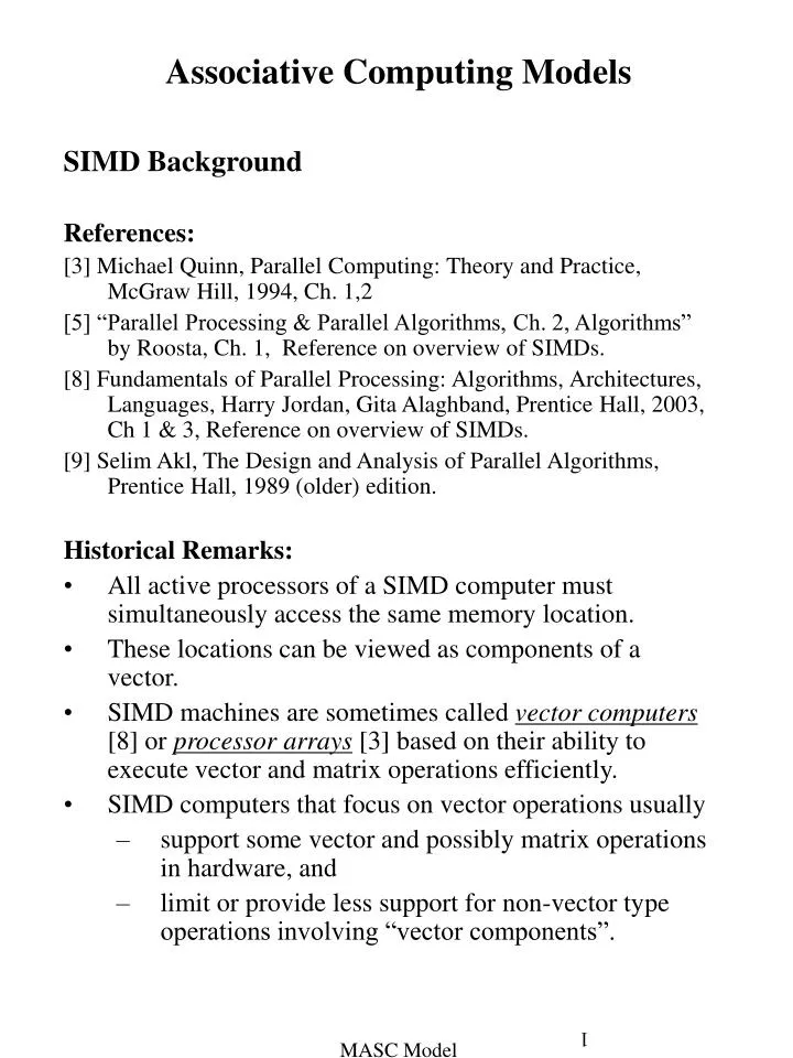
Busy- idle On lot Color Model Price Year Make PE1 1 red Dodge 1 1994 0 PE2 0 PE3 1 blue 1996 Ford 1 IS PE4 0 1 1998 white Ford PE5 0 0 PE6 0 0 1 1 Subaru PE7 1997 red The Associative Search MASC Model
Characteristics of Associative Programming • Consistent use of data parallel programming • Consistent use of global associative searching & responder processing • Regular use of the constant time global reduction operations: AND, OR, MAX, MIN • Broadcast of data using IS bus (and IS fork and join operations for MASC) allows the use of the PE network to be restricted to parallel data movement. • Tabular representation of data • Use of searching instead of sorting • Use of searching instead of pointers • Use of searching instead of ordering provided by linked lists, stacks, queues • Promotes an intuitive style of programming that promotes high productivity • Uses structure codes (i.e., numeric representation) to represent data structures such as trees, graphs, embedded lists, and matrices. • See Nov. 1994 IEEE Computer article. • Also, see “Associative Computing” [11,Potter]. MASC Model
Languages Designed for MASC • The ASC language was designed by Jerry Potter for MASC(n,1) (or ASC). • Based on C and Pascal • Initially designed as a parallel language. • Avoids compromises required to extend an existing sequential language • E.g., avoids unneeded sequential constructs such as pointers • Implemented on several SIMD computers • Goodyear Aerospace’s STARAN • Goodyear/Loral’s ASPRO • Thinking Machine’s CM-2 • WaveTracer • ACE is a higher level language that uses natural language syntax; e.g., plurals, pronouns. • Anglish is an ACE variant that uses an English-like grammar (e.g., “their”, “its”) • An OOPs version of ASC for MASC(n,k) is planned (by Potter and his students) • Language References: • ASC Primer • “Associative Computing” book by Potter [11] • Our parallel website • www.mcs.kent.edu/~potter/ MASC Model
Algorithms and Programs Implemented in ASC or MASC • A wide range of algorithms implemented in ASC (and a few in MASC) without use of PE network • ASC Graph Algorithms • minimal spanning tree • IEEE COMPUTER paper on ASC. • shortest path • Similar to MST • connected components • Project by Scherger. Similar to MST • ASC/MASC Computational Geometry Algorithms • convex hull algorithms (Jarvis March, Quickhull, Graham Scan, etc) • Dynamic hull algorithms • Reference: Maher Atwah thesis & dissertation. Most in PDCS or WMPP papers that are on our parallel website. • ASC String Matching Algorithms • all exact substring matches • all exact matches with “don’t care” (i.e., wild card) characters. • Reference: 1995 thesis by Mary Esenwein and PDCS paper on our parallel website. MASC Model
(cont.) ASC/MASC Algorithms & Programs • Algorithms for NP-complete problems • Traveling salesperson • ASC algorithm and STARAN program • Thesis by Julie Lee in 1989 • Not submitted for publication • 2-D knapsack algorithm in ASC • Dissertation by Darrell Ulm and an ICPP conference paper on our parallel website. • 2D knapsack algorithm in MASC • Darrell Ulm, to appear in 2004 WMPP Workshop. Also on our parallel website. • Regular 0/1 Knapsack Problem • Constant time ASC algorithm using an exponential number of PEs • Also STARAN program • Thesis by Steven Talus in 1988. • Data Base Management Software • associative data base • relational data base • Theses sponsored by Potter and Meilander starting in mid or late l980’s. MASC Model
(Cont) ASC Algorithms and Programs • A Two Pass Compiler for ASC (first pass and • first pass and optimization phase • Thesis by Chandra Asthagiri (sponsored by Jerry Potter) - probably late 1980’s • Used by Potter in ASC language. • Two Rule-Based Inference Engines • OPS-5 interpreter • Thesis by Tim Haston & sponsored by Potter – probably in late 1980’s • PPL (Parallel Production Language interpreter) • Thesis by Andrew Miller & sponsored by Baker – probably late 1980’s. • Paper published in Frontiers MMP conference. • A Context Sensitive Language Interpreter • (OPS-5 variables force context sensitivity) • Thesis work by Chandra Asthagiri or Tim Haston & sponsored by Potter – probably in late 1980. • An associative PROLOG interpreter • Work by Jerry Potter and Arvind Bansal • Published and also probably in thesis. MASC Model
Programs in ASC - Using a PE Network • 2-D Knapsack Algorithm using a 1-D mesh • Reference to be added • Image Processing algorithms using 1-D mesh • Some algorithms in Potters book • Probably some in papers published by Potter • Possibly some in Goodyear Aerospace in-house algorithms (we may have draft version) • FFT using Flip Network • In-house algorithms from Goodyear Aerospace • We have a draft version. • Matrix Multiplication using 1-D mesh • In house algorithms from Goodyear Aerospace • We may have a draft version of some of these • An Air Traffic Control Program (using Flip network connecting PEs to memory) • Demonstrated using live data at Knoxville in mid 70’s. • Paper on Air Traffic Control by Meilander, Jin, and Baker in 2002 PDCS conference & on our parallel website. • Multiple papers with Will Meilander published in both professional & trade conferences or journals. (Some on our parallel website) • Several thesis sponsored by Will Meilander (and usually Baker). • Undefended thesis by Jinjin Xie, 2000. MASC Model
Preliminaries for ASC Algorithm for MST • Next, a “data structure” level presentation of Prim’s algorithm for the MST is given. • The data structure used is illustrated in the next two slides. • This example is from [10] in Nov. 1994 IEEE Computer. • There are two types of variables for the ASC model, namely • the parallel variables (i.e., ones for the PEs) • the scalar variables (ie., the ones for the control unit). • Scalar variables are essentially global variables. • Can replace each with a parallel variable. • To aid in distinguishing between them, the parallel variables names end with a “$” symbol. • Each step in this algorithm is constant. • One MST edge is selected during each pass through the loop in this algorithm. • Since a spanning tree has n-1 edges, the running time of this algorithm is O(n). • Since the sequential running time of the Prim MST algorithm is O(n 2) and is time optimal, this parallel implementation is cost optimal. MASC Model
a 2 2 8 7 b c 4 3 9 6 e d 3 f Figure 6 in [10, Potter, Baker, et. al.] MASC Model
candidate$ current_best$ mask$ node$ parent$ PEs d$ c$ b$ e$ f$ a$ a ∞ 2 8 ∞ ∞ ∞ no b 2 ∞ 7 4 3 ∞ no a 2 c 8 7 ∞ ∞ 6 9 yes b 7 IS sequential program control d ∞ 4 ∞ ∞ 3 ∞ yes b 4 a e ∞ 3 6 3 ∞ ∞ yes b 3 root b f ∞ ∞ 9 ∞ ∞ ∞ wait next- node MASC Model
Algorithm: ASC-MST-PRIM(root) • Initialize candidates to “waiting” • If there are any finite values in root’s field, • set candidate$ to “yes” • set parent$ to root • set current_best$ to the values in root’s field • set root’s candidate field to “no” • Loop while some candidate$ contain “yes” • for them • restrict mask$ to mindex(current_best$) • set next_node to a node identified in the preceding step • set its candidate to ‘no” • if the values in next_node’s field are less than current_best$, then • set current_best$ to value in next_node’s field • set parent$ to next_node • if candidate$ is “waiting” and the value in next_node’s field is finite • set candidate$ to “yes” • set parent$ to next_node • set current_best to the values in next_node’s field Figure 6(c) in [10, Potter, Baker, et. al.] MASC Model
Comments on Figure 6 • The three preceding slides show figure 6 from [10, IEEE Computer, Nov 1994]. • Figure 6c gives a compact, data-structures level pseudo-code description for this algorithm • Pseudo-code illustrates Potter’s use of pronouns (e.g., them) • The mindex function returns the index of a processor holding the minimal value. • This MST pseudo-code is much simpler than data-structure level sequential MST pseudo-codes (e.g., Sara Baase’s textbook [13] below.) • We will next see a more detailed explanation of the algorithm in Figure 6c. [13] Sara Baase, Computer Algorithms: Introduction to Design and Analysis, 2nd Edition, Addison Wesley Publishing Co.,1988, 162-166. MASC Model
Algorithm: ASC-MSP-PRIM • Initially assign any node to root. • All processors initialize the following variables: • candidate$ to “waiting” • current-best$ to • the candidate fieldfor the root node to “no” • All processors whose distance d from their node to root node is finite do • Set their candidate$ field to “yes • Set their parent$ field to root. • Set current_best$ = d. • While the candidate field of some processor is “yes”, • Restrict the active processors to those responding and (for these processors) do • Compute the minimum value x of current_best$. • Restrict the active processors to those with current_best$ = x and do • pick an active processor, say one with node y. • Set the candidate$ value of node y to “no” • Set the scalar variable next-node to y. MASC Model
If the value z in the next_node column of a processor is less than its current_best$ value, then • Set current_best$ to z. • Set parent$ to next_node • For all processors, if candidate$ is “waiting” and the distance of its node from next_node is finite, then • Set candidate$ to “yes” • Set parent$ to next-node • Set current_best$ to the distance of its node from next_node. MASC Model
h e w Quickhull Algorithm for ASC • Reference: • [14, Maher, et.al, Associative Convex Hull] • Review of Sequential Quickhull Algorithm • Suffices to find the upper convex hull of points in below diagram that are on are above line . • Select point h so that the area of triangle weh is maximal. • Proceed recursively with the sets of points on or above the lines and . MASC Model
point$ y-coord$ left-point$ x-coord$ right-pt$ job$ area$ name$ hull$ p1 1 3 p1 p3 1 1 w 0 p2 7 1 p1 p3 0 IS 12 2 p1 p3 1 1 e p3 p4 8 4 p1 p3 1 p5 11 7 p1 p3 1 h ctr h p6 8 9 p1 p3 1 1 p7 2 6 p1 p3 1 P6, h p5 p7 p4 p1, w P3, e p2 MASC Model
ASC Quickhull Algorithm(Upper Convex Hull) ASC-Quickhull( planar-point-set ) • Initialize: ctr = 1, area$ = 0, hull$ = 0 • Find the PE with the minimal x-coord$ and let w be its point$ • Set its hull$ value to 1 • Find the PE with the PE with maximal x-coord$ and let e be its point$ • Set its hull$ to 1 • All PEs set their left-pt to w and right-pt to e. • If the point$ for a PE lies above the line • Then set its job$ value to 1 • Else set its job$ value to 0 MASC Model
ASC Quickhull (continued) • Loop while parallel job$ contains a nonzero value • The IS makes its active cell those with a maximal job$ value. • Each active PE computes & stores in area$ the area of triangle( left-pt$, right-pt$, point$ ) • Find the PE with the maximal area$ and let h be its point. • Set its hull$ value to 1 • Each active PE whose point$ is above sets its job$ value to ++ctr • Each active PE whose point$ is above sets its job$ to ++ctr • Each active PE with job$ < ctr -2 sets its job$ value to 0 MASC Model
5 3 1 4 2 6 0 Performance of ASC-Quickhull Average Case: • Assume • roughly of the points above each line being processed are eliminated. • O(lg n) points are on the convex hull. • Then the average running time is O(lg n) • The average cost is O(n lg n) Worst Case: • Running time is O(n). • Cost is O(n2) Figure: Processing Order for Areas MASC Model
MASC Quickhull Algorithm(Upper Convex Hull) Algorithm: • Use IS1 to execute the first loop of ASC-Quickhull • Idle ISs request problems from busy ISs who have inactive jobs on their job$ list. • Control of the PEs for an inactive job are transferred to the idle IS. The control of these PEs is returned to original IS after the job is finished. 2 2 1 1 2 2 0 MASC Model
Analysis for MASC Quicksort Average Case: • Assumptions: • roughly of the points above each line being processed are eliminated. • O(lg n) Instruction Streams are available. • There are O(lg n) convex hull points • The average running time is O(lg lg n) • Essentially constant time for real world problems. Worst Case • O(n) Note: Taken from a latex presentation prepared by Atwah called “An Associative Model of Computation” in directory ~jbaker/slides/matwah. MASC Model
Simulations Between MASC and MMB • The reference for these results is the paper by Baker and Jin, Simulation of Enhanced Meshes with MASC, a MSIMD Model, Proc of the IASTED Internatl Conf on Parallel and Distributed Computing Systems, Nov 1999, 511-516. • Enhanced meshes are basic mesh models augmented with fixed or reconfigurable buses • At most one PE on a bus can broadcast to remaining PEs during one step. • The best-known fixed bus example is the Mesh with multiple broadcasting (MMB) • Standard 2-D mesh • Row and column bus enhancements • Broadcasts can occur along only row or column buses (but not both) in one step MASC Model
Simulation Preliminaries • Reasons to simulate other models using MASC • Allows a better understanding of the power of MASC • Provides a simulation algorithm that permits algorithms designed for the simulated model to run on MASC • Basic Assumption Used in the Simulations • MASC(n, ) has a mesh PE network with row-major ordering • The enhanced meshes have a 2D mesh with the same size and ordering • Each PE in MASC has the same computational power as an enhanced mesh PE • The MASC buses and the buses of the enhanced mesh have the same characteristics • The word lengths of both models are the same and at least lg(n). • Each PE in MASC knows its position in the 2D mesh. • Each of the MASC PEs can store its position coordinates in two words. MASC Model
I S N e t w o r k IS2 IS IS1 ·· · · · j Cell Cell Cell · · · · · · · · · · Cell Cell Cell C e l l N e t w o r k Simulation Mappings between MASC & the Enhanced Mesh MMB • The mapping is between MASC(n, ) and an enhanced mesh of size . • The mapping assigns a PE in one model to the PE that is in the same position in the 2D mesh in the other model • The ith IS in MASC simulates both the ith row and the ith column buses · MASC Model
Simulation of MMB with MASC • Since both models have identical 2D meshes, these do not need to be simulated • Since the power of PEs in respective models are identical, their local computations are not simulated • To simulate a MMB row broadcast on the MASC, • All PEs switch to their assigned row IS • The IS for each row checks to see if there is a PE that wishes to broadcast • If true, the IS broadcasts this value to all of its PEs (i.e., the ones on its assigned row). • Simulation of a MMB column broadcast is similar • The running time is O(1). Theorem 1 • MASC(n, j) with a 2-D mesh and j = ( ) can simulate a MMB in constant time. • An algorithm for a MMB can be executed on MASC(n, j) with j=( ) and a 2-D mesh with a running time at least fast as the MMB time. MASC Model
Simulation of MASC by MMB • PE(1,1) stores a copy of the program and simulates the ISs sequentially. • Each instruction stream command or datum is first sent by P(1,1) to the PEs in the first column. • Next, all PEs in the first column broadcast this command or datum to all PEs on their row. • Each MMB processor uses two registers, channel and status, to decide whether or not to execute the current instruction. • channel records the IS to which each PE is assigned. • status records whether PE is active, inactive, idle • The simulation of simultaneous broadcasts of ISs takes O( ) time. • A local computation, memory access, or a data movement along local links are identical in the two models and require O(1) time. • The execution of a global reduction operator OR, AND, MAX, MIN takes O( ) using an optimal MMB algorithm (see reference paper) • Note this means MASC is more powerful. • Since the global reduction operators might have to be computed for O( ) ISs, an upper bound for the simulation is O( ) = O( ). MASC Model
Theorem 3. • MASC(n, ) with a 2-D mesh can be simulated by a MMB in O( ) time with O( ) extra memory Example • Assume that an matrix A is stored in a mesh with one value in each PE. • Consider a partition of A into sets A1, A2, ... , A so that each Aj contains exactly one value of A from each column and each row. • An example of such a partition can be obtained using the wrap-around diagonals of this table. • The MASC(n, ) architecture can find the maximum of all of the Ai sets in parallel in O(1) time by having the PEs with data in Ailisten to ISi. • A MMB requires ( log n) time to do calculation since • The calculation of each maximum on MMB requires O(lg n) time (See reference paper) • The buses can only calculate each maximum serially. THEOREM 4. • MASC(n, j) with a 2-D mesh is strictly more powerful than a MMB for j = ( ). MASC Model
Conclusion • MASC is strictly more powerful than an MMB of the same size. • Any algorithm for an MMB can be executed on a MASC of the same size with the same running time. In particular, • Optimal algorithms for MMB are also optimal when executed on MASC • CLAIM: MASC and RM are dissimilar and can not simulate each other efficiently. • DISCUSSION: • Cost of the MASC simulation of MMB. MASC Model
Unused Slides Follow MASC Model
The Reconfigurable Enhanced Mesh RM • For all reconfigurable bus models, buses are created dynamically during execution • Best known example: • General Reconfigurable Mesh (RM) • Each PE has four ports called N,S, E, W (often called “NEWS”) • In one step, each PE can set the connections of its ports, based on local data • At most two disjoint pairs of ports can be connected at any time • One such connection is the adjacent pairs, {{N,E}, {W,S}}. MASC Model