Download

1 / 20
200 likes | 337 Views
Measuring Magnetoresistance and Bulk Magnetization in Pulsed Magnetic Fields. Charles Bosse. BT&T Organic Semiconductors Group. Pulsed Magnets. Reach high field Relatively low power consumption Rapid Field transition Noise in data Magnets eventually explode. Front. Back.

E N D
Measuring Magnetoresistance and Bulk Magnetization in Pulsed Magnetic Fields Charles Bosse BT&T Organic Semiconductors Group
Pulsed Magnets • Reach high field • Relatively low power consumption • Rapid Field transition • Noise in data • Magnets eventually explode
Front Back 27 T Pulsed Magnet and Cryostat • Low cost magnet • Short pulse (15 msec) • 8 msec rise time • Low temperature (about 2 K) Cryostat G10 Vacuum Jacket Probe tip LN2 LHe Magnetoresistance Sample Stage Probe Thermometer Magnet Magnetization Kapton and stainless steel foil tail coil Magnetization sample inside coil
Magnetoresistance • Magnetoresistance is the effect of increase in resistance in a conductor with increase in magnetic field. • Different behavior at different temperatures. • Studied two materials: Bi and (TMTSF)2AsF6
Why Bismuth • Known to have measurable magnetoresistance at liquid nitrogen temperatures • Previous study makes it a good comparison material
Bismuth Results • Resistance vs. Field at 77 K shows standard increase of resistance over field . • Quantum Oscillations at liquid helium temperatures are caused by closed orbits of electrons at the Fermi surface so that electrons can only follow certain paths.
What is (TMTSF)2AsF6? • TMTSF (tetramehyl tetraselenefulvalene ) is the main component of a series of compounds known as Bechgaard salts. These salts are organic metals, or conductive organic structures, and some of them show superconductive or semiconductive properties. • TMTSF-AsF6 is is a “ quasi one-dimensional” conductor: it has dramatically different current carrying characteristics depending on the orientation.
Why examine the magnetoresistance of (TMTSF)2AsF6? • Electrons are mostly confined to one dimensional movement at low temperatures. This means the material should switch to being mostly insulating at low temperature and mid to high field as the magnetic field tries to push electrons across unavailable states perpendicular to the plain of conduction. • A less widely studied but still interesting material.
Results for (TMTSF)2AsF6 MR • Temperature curve shows “insulator” transition at 12 K • MR Data Shows interesting trend – worth further study
Measuring Magnetization • In a two-coil system, with one coil wound in reverse of the other, one induced current will cancel if the coils are centered. • Possible to measure the change in magnetism in a material centered in one of the two coils. • Magnetism of material will distort field and allow more or less induced current in one coil, resulting in a measurable net imbalance.
Mn12-acetate, a molecular magnet • Mn12-acetate is a high spin molecular magnet within a crystal lattice. • Consists of eight spin up and four spin down systems with quantized orientations. • Quantized orientation result in hysteresis in Mn12-Acetate is stair-stepped instead of following the normal “bird shaped” pattern. • Stair stepping depends on speed of field change B. Barbara “Macroscopic quantum tunneling in molecular magnets, JMMM 200 (1999) 167}181
Observed Magnetization in Mn12-acetate B. Barbara “Macroscopic quantum tunneling in molecular magnets, JMMM 200 (1999) 167}181 • All previous data has been taken in SQUIDS, transition a few Tesla per hour, where the pulse magnet transitions a few Tesla per millisecond. • Hoped to find transitions- Inconclusive due to noise problem, needs further calibration
Advantages and Disadvantages of mid-strength low cost pulse magnets • Advantages: • Cheap, small, relatively low power use, able to withstand very low temperatures, rapid field change, good for high field data that can be taken in a short time • Disadvantages: • low signal to noise, sometimes flaky at low temp, signal needs preamp, sample in direct contact with cryogens
James Brooks, David Graf, Noppi Widjaja, Eun Sang Choi, Relja Vasic, Eric Jo, Jin Geou, Jean Christoph, Yugo Oshima, Takahisa Tokumoto Special Thanks to the BTT Lab
Heartfelt thanks also to the CIRL staff: Gina LaFrazza Dave Sheaffer Pat Dixon Stacy Vanderlaan Carlos Villa 29
And finally, • To the National High Magnetic Field Lab, the National Science Foundation, for the funding to support this program and make it possible
Measurement Technique • Four terminal measurement • V=IR so with a constant current, if voltage changes, resistance changes. • Measure Voltage on oscilloscope vs. time
Finding Magnetic Field calculating field from induced voltage in the pick-up coil: The induced voltage in a coil comes the rate of change of the flux: Eq. 1 The flux through a given loop depends on the strength of the field and open loop area: Eq. 2 Combining equations 1 and 2 we have: (re-arrange equation) where…. A = open loop area: pr2*n n = # of turns in the coil: 10 e = induced voltage in the coil: measured by scope F = magnetic flux B = magnetic field • Function integreat() • variable i, A,N, bsum, offset • A = pi*((6.35e-3)/2)^2 • N = 10 • offset = -.0075 • bsum=0 • i = 0 • do • bsum = bsum + (VPu3[i+1] + VPu3[i] + offset*2)*(time03[i+1] - time03[i])/2/(N*A) • B03[i]= bsum • I+=1 • while(i<49995) • end • Function integreatMAG() • variable i, bsum, offset1, offset2 • |A = pi*((6.35e-3)/2)^2 • |N = 10 • offset1 = 0 • offset2 = 1 • bsum=0 • i = 0 • do • bsum = bsum + (NC05zero[i+1] + NC05zero[i] + offset1)*(time05[i+1] - time05[i])/(offset2) • MagMC005[i]= bsum • I+=1 • while(i<49995) • end