Download
1 / 24
240 likes | 320 Views
Learn how to create and interpret graphs in Saturn, conduct multiple linear regression, control for confounding variables, and explore interactions in statistical analysis using SAS software. Understand significance testing and coefficients in regression analysis.

E N D
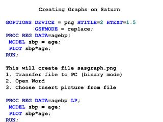
Creating Graphs on Saturn • GOPTIONSDEVICE = png HTITLE=2HTEXT=1.5 • GSFMODE = replace; • PROCREGDATA=agebp; • MODEL sbp = age; • PLOT sbp*age; • RUN; • This will create file sasgraph.png • Transfer file to PC (binary mode) • 2. Open Word • 3. Choose Insert picture from file • PROCREGDATA=agebp LP; • MODEL sbp = age; • PLOT sbp*age; • RUN;
Multiple Linear Regression • More than 1 independent variable • See how combinations of several variables are associated with and can predict the dependent variable. How much of the total variability can be explained? • Control for confounding (interested in the effect of one variable but want to “adjust” for another variable) • Explore interactions PROCREG DATA=datasetname; MODELdepvar = x1; MODELdepvar = x1 x2; MODELdepvar = x1 x2 x3; RUN;
Question Explored Using Multiple Regression • How much of the variation in test scores among school districts can be explained by several district characteristics? • Is calcium intake related to BP independent of age? • Is the relationship between age and BP the same for men and women.
Reminder • Y variable is continuous and is normally distributed for each combination of X’s with the same variability • X variables can be continuous or indicator variables and do not need to be normally distributed
2 Factors • Y = b0 + b1X1 • Y = b0 + b2X2 • Y = b0 + b1X1 + b2X2 • Do you get the same slope in models 1 and 3
Control for confounding Both SLR models for each cohort significant Overall not significant (negative confounding)
Multiple Regression Equation • The equation that describes how the mean value of y is related to x1, x2, . . . xp . my = 0 + 1x1 + 2x2 + . . . + pxp b0=Mean of y when all x variables are equal to 0 bi = change in mean y corresponding to a 1 unit change in xi considering all other predictors fixed Implied: The impact of x1 is the same for each of the other values of x2, x3, … xp
Multiple Regression Model • The equation that describes how the dependent variable y is related to the independent variables x1, x2, . . . xp and an error term is called the multipleregression model. y = b0 + b1x1 + b2x2 +. . . + bpxp + e ereflects how individuals deviate from others with the same values of x’s
Estimated Multiple Regression Equation • The estimated multiple regression equation is: y = b0 + b1x1 + b2x2 + . . . + bpxp ^ bi estimates bi yis estimated (or predicted) value for a set of x’s ^
Estimation • Least Squares Criterion • Computation of Coefficients Values The formulas for the regression coefficients b0, b1, b2, . . . bp involve the use of matrix algebra. We will use SAS to perform the calculations. ^
Testing for Significance: Global Test • Hypotheses H0: 1 = 2 = . . . = p = 0 Ha: One or more of the parameters is not equal to zero. • Test Statistic F = MSR/MSE • Rejection Rule Reject H0 if F > F where F is based on an F distribution with p d.f. in the numerator and n - p - 1 d.f. in the denominator.
Testing for Significance: Individualb’s • Hypotheses H0: i = 0 Ha: i = 0 • Test Statistic • Rejection Rule Reject H0 for small or large t Meaning: Is Xi related to Y after taking into account all other variables in the model
Possibilities • X1 is related to Y alone but after adjusting for X2, then X1 is no longer related to Y • X1 is not related to Y alone but after adjusting for X2, then X1 is related to Y • Relation of X1 with Y1 gets stronger after adjusting for X2 • Relation of X1 with Y gets weaker after adjusting for X2
Pulmonary Function Example • Dependent Variable: Forced Expired Volume (FEV1.0) • Independent Variables: • Age of person • Smoking status of person • Questions: • Is age related to FEV independent of smoking status • Is smoking status related to FEV independent of age • How much of the variability in FEV is explained by age and smoking combined
Model for FEV Example Y = b0 + b1X1 + b2X2 X1 = smoking status (1=smoker, 0=nonsmoker) X2 = age Smokers FEV = b0 + b1 + b2age Non Smokers FEV = b0 + b2age
Interpretation of Parameters Smokers FEV = b0 + b1 + b2age Non Smokers FEV = b0 + b2age b1 is the effect of smoking for fixed levels of age b2 is the effect of age pooled over smokers and non-smokers This model assumes the relation of age to FEV is the same for smokers and non-smokers
DATA fev; INFILE DATALINES; INPUT age smk fev; DATALINES; 28 1 4.0 30 1 3.9 30 1 3.7 31 1 3.6 54 0 2.9 More data
PROCMEANS; VAR fev; CLASS smk; RUN; The MEANS Procedure Analysis Variable : fev N smk Obs N Mean Std Dev Minimum Maximum 0 15 15 3.6000000 0.4208834 2.9000000 4.3000000 1 15 15 3.2933333 0.5257195 2.2000000 4.000000
PROCCORR DATA=fev; Pearson Correlation Coefficients, N = 30 Prob > |r| under H0: Rho=0 age smk fev age 1.00000 -0.12788 -0.73024 0.5007 <.0001 smk -0.12788 1.00000 -0.31620 0.5007 0.0887 fev -0.73024 -0.31620 1.00000 <.0001 0.0887
PROCREG; MODEL fev = age smk ; RUN; Dependent Variable: fev Analysis of Variance Sum of Mean Source DF Squares Square F Value Pr > F Model 2 SSR 4.96510 2.48255 32.08 <.0001 Error 27 SSE 2.08957 0.07739 Corrected Total 29 SST 7.05467 Root MSE 0.27819 R-Square 0.7038 Dependent Mean 3.44667 Coeff Var 8.07136 Tests Ho: b1 = 0; b2 =0 Proportion of variance explained by both variables
PROCREG; MODEL fev = age smk ; MODEL fev = age ; MODEL fev = smk ; RUN; Parameter Estimates Parameter Standard Variable DF Estimate Error t Value Pr > |t| Intercept 1 5.58114 0.27653 20.18 <.0001 age 1 -0.04702 0.00634 -7.42 <.0001 smk 1 -0.40384 0.10242 -3.94 0.0005 Intercept 1 5.24787 0.32456 16.17 <.0001 age 1 -0.04382 0.00775 -5.66 <.0001 Intercept 1 3.60000 0.12295 29.28 <.0001 smk 1 -0.30667 0.17388 -1.76 0.0887 R2 = .7038 R2 = .5333 R2 = .1000
PROCREG; MODEL fev = age smk; PROCREG; MODEL fev = age ; WHERE smk = 0; PROCREG; MODEL fev = age ; WHERE smk = 1; Parameter Standard Variable DF Estimate Error t Value Pr > |t| Intercept 1 5.58114 0.27653 20.18 <.0001 age 1 -0.04702 0.00634 -7.42 <.0001 smk 1 -0.40384 0.10242 -3.94 0.0005 Parameter Standard Variable DF Estimate Error t Value Pr > |t| Intercept 1 5.24764 0.38050 13.79 <.0001 age 1 -0.03911 0.00887 -4.41 0.0007 Intercept 1 5.50002 0.36163 15.21 <.0001 age 1 -0.05508 0.00885 -6.22 <.0001 Non-smokers Smokers