Download
1 / 132
1.37k likes | 1.58k Views
Sampling and Reconstruction. Digital Image Synthesis Yung-Yu Chuang. with slides by Pat Hanrahan, Torsten Moller and Brian Curless. Sampling theory.

E N D
Sampling and Reconstruction Digital Image Synthesis Yung-Yu Chuang with slides by Pat Hanrahan, Torsten Moller and Brian Curless
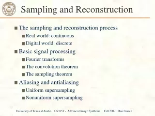
Sampling theory • Sampling theory: the theory of taking discrete sample values (grid of color pixels) from functions defined over continuous domains (incident radiance defined over the film plane) and then using those samples to reconstruct new functions that are similar to the original (reconstruction). Sampler: selects sample points on the image plane Filter: blends multiple samples together
Aliasing • Reconstruction generates an approximation to the original function. Error is called aliasing. sampling reconstruction sample value sample position
Sampling in computer graphics • Artifacts due to sampling - Aliasing • Jaggies • Moire • Flickering small objects • Sparkling highlights • Temporal strobing (such as Wagon-wheel effect) • Preventing these artifacts - Antialiasing
Jaggies Retort sequence by Don Mitchell Staircase pattern or jaggies
Moire pattern • Sampling the equation
Fourier analysis • Can be used to evaluate the quality between the reconstruction and the original. • The concept was introduced to Graphics by Robert Cook in 1986. (extended by Don Mitchell) • Rob Cook • V.P. of Pixar • 1981 M.S. Cornell • 1987 SIGGRAPH Achievement • award • 1999 Fellow of ACM • Academic Award with • Ed Catmull and Loren • Carpenter (for Renderman)
Fourier transforms • Most functions can be decomposed into a weighted sum of shifted sinusoids. • Each function has two representations • Spatial domain - normal representation • Frequency domain - spectral representation • The Fourier transform converts between the spatial and frequency domain Spatial Domain Frequency Domain
Fourier analysis spatial domain frequency domain
Fourier analysis spatial domain frequency domain
Fourier analysis spatial domain frequency domain
Convolution • Definition • Convolution Theorem: Multiplication in the frequency domain is equivalent to convolution in the space domain. • Symmetric Theorem: Multiplication in the space domain is equivalent to convolution in the frequency domain.
2D convolution theorem example f(x,y) g(x,y) h(x,y) F(sx,sy) G(sx,sy) H(sx,sy)
The delta function • Dirac delta function, zero width, infinite height and unit area
Shah/impulse train function spatial domain frequency domain ,
Sampling band limited
Reconstruction The reconstructed function is obtained by interpolating among the samples in some manner
Reconstruction filters The sinc filter, while ideal, has two drawbacks: • It has a large support (slow to compute) • It introduces ringing in practice The box filter is bad because its Fourier transform is a sinc filter which includes high frequency contribution from the infinite series of other copies.
Aliasing decrease sample spacing in frequency domain increase sample spacing in spatial domain
Aliasing high-frequency details leak into lower-frequency regions
Sampling theorem • For band limited functions, we can just increase the sampling rate • However, few of interesting functions in computer graphics are band limited, in particular, functions with discontinuities. • It is mostly because the discontinuity always falls between two samples and the samples provides no information about this discontinuity.
Aliasing • Prealiasing: due to sampling under Nyquist rate • Postaliasing: due to use of imperfect reconstruction filter
Antialiasing • Antialiasing = Preventing aliasing • Analytically prefilter the signal • Not solvable in general • Uniform supersampling and resample • Nonuniform or stochastic sampling
It is blurred, but better than aliasing
Uniform supersampling • Increasing the sampling rate moves each copy of the spectra further apart, potentially reducing the overlap and thus aliasing • Resulting samples must be resampled (filtered) to image sampling rate Samples Pixel
Point vs. Supersampled Point 4x4 Supersampled Checkerboard sequence by Tom Duff
Analytic vs. Supersampled Exact Area 4x4 Supersampled
Non-uniform sampling • Uniform sampling • The spectrum of uniformly spaced samples is also a set of uniformly spaced spikes • Multiplying the signal by the sampling pattern corresponds to placing a copy of the spectrum at each spike (in freq. space) • Aliases are coherent (structured), and very noticeable • Non-uniform sampling • Samples at non-uniform locations have a different spectrum; a single spike plus noise • Sampling a signal in this way converts aliases into broadband noise • Noise is incoherent (structureless), and much less objectionable • Aliases can’t be removed, but can be made less noticeable.
Antialiasing (nonuniform sampling) • The impulse train is modified as • It turns regular aliasing into noise. But random noise is less distracting than coherent aliasing.
Jittered vs. Uniform Supersampling 4x4 Jittered Sampling 4x4 Uniform
Prefer noise over aliasing reference aliasing noise
Jittered sampling Add uniform random jitter to each sample
Poisson disk noise (Yellott) • Blue noise • Spectrum should be noisy and lack any concentrated spikes of energy (to avoid coherent aliasing) • Spectrum should have deficiency of low-frequency energy (to hide aliasing in less noticeable high frequency)
Distribution of extrafoveal cones Monkey eye cone distribution Fourier transform Yellott theory • Aliases replaced by noise • Visual system less sensitive to high freq noise
Aliasing function (a) function (b) frequency domain alias=false frequency
Stochastic sampling function (a) function (b) Replace structure alias by structureless (high-freq) noise
Antialiasing (adaptive sampling) • Take more samples only when necessary. However, in practice, it is hard to know where we need supersampling. Some heuristics could be used. • It only makes a less aliased image, but may not be more efficient than simple supersampling particular for complex scenes.
Application to ray tracing • Sources of aliasing: object boundary, small objects, textures and materials • Good news: we can do sampling easily • Bad news: we can’t do prefiltering (because we do not have the whole function) • Key insight: we can never remove all aliasing, so we develop techniques to mitigate its impact on the quality of the final image.
pbrt sampling interface • Creating good sample patterns can substantially improve a ray tracer’s efficiency, allowing it to create a high-quality image with fewer rays. • Because evaluating radiance is costly, it pays to spend time on generating better sampling. • core/sampling.*, samplers/* • random.cpp, stratified.cpp, bestcandidate.cpp, lowdiscrepancy.cpp,