Download
1 / 21
210 likes | 426 Views
Sampling, Reconstruction, and Elementary Digital Filters. R.C. Maher ECEN4002/5002 DSP Laboratory Spring 2003. Sampling and Reconstruction.

E N D
Sampling, Reconstruction, and Elementary Digital Filters R.C. Maher ECEN4002/5002 DSP Laboratory Spring 2003
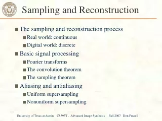
Sampling and Reconstruction • Need to understand relationship between a continuous-time signal f(t) and a discrete-time (sampled) signal f(kT), where T is the time between samples (T=1/fs) Delay Lines and Simple Filters R. C. Maher
Sampling (cont.) • After some manipulation, can show: Delay Lines and Simple Filters R. C. Maher
Xc(j) -N N XS(j) -2S -S -N N S 2S Sampling Effects: Frequency Domain Fourier Transform of continuous function Fourier Transform of sampled function S > 2 N S < 2 N (aliasing) XS(j) -2S -S S 2S Delay Lines and Simple Filters R. C. Maher
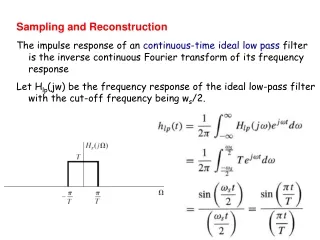
XS(j) -2S -S -N N S 2S Reconstruction • Since spectrum of sampled signal consists of baseband spectrum and spectral images shifted at multiples of 2π/T, reconstruction means isolating the baseband image • Concept: lowpass filter to pass baseband while removing images Delay Lines and Simple Filters R. C. Maher
Reconstruction (cont.) • Multiplication by rectangular pulse in frequency domain (LPF) corresponds to convolution by sinc( ) function in time domain • Because sinc( ) is non-causal and of infinite extent, practical reconstruction requires an approximation to the ideal case Delay Lines and Simple Filters R. C. Maher
Delay Lines • In order to create a frequency-selective function, there must be a delay memory so that the function is able to observe and resolve the frequencies present in the signal • Digital filters used tapped delay lines to create the z-1 (delay) terms in the z-transform Delay Lines and Simple Filters R. C. Maher
+ x[n] y[n] h0 Z-1 x[n-1] h1 Z-1 x[n-2] h2 Z-1 x[n-3] h3 Delay Lines (cont.) Delay Lines and Simple Filters R. C. Maher
Delay Lines (cont.) • Delay lines can be implemented easily as a one dimensional array or FIFO in DSP memory • Typically use an address register to point to array, then just increment pointer instead of copying data to achieve the delay Delay Lines and Simple Filters R. C. Maher
Modulo Buffers • DSP supports modulo arithmetic in the address generation unit • With modulo buffer, incrementing or decrementing address register “rolls over” automatically at beginning and ending of buffer memory range • Modulo buffers are useful for delay stages in filters and other FIFO queue structures Delay Lines and Simple Filters R. C. Maher
Base Address + N -1 N memory locations Modulo N Buffer Memory Base Address Modulo Buffers (cont.) • Modulo calculations keep address pointer within a fixed range of memory locations Delay Lines and Simple Filters R. C. Maher
56300 Modulo Buffers • The M registers in the AGU select the modulo size of the buffer • M = $FFFFFF implies no modulo (regular linear addressing) • M = 0 implies bit-reversed addressing (useful in FFT algorithms) • M = ‘modulo’-1 implies address range including ‘modulo’ memory locations (2modulo $7FFF) Delay Lines and Simple Filters R. C. Maher
56300 Modulo (cont.) • The base address of the modulo buffer must be a power of 2 • The base address must either be zero, or a power of 2 that is greater than or equal to the modulo • In other words, the base address must be 2k, where 2kmodulo, which implies k least significant bits must be zero Delay Lines and Simple Filters R. C. Maher
FIR Filter • FIR filter coefficients are equal to the unit sample response of the filter • Given filter specifications, we need to choose a unit sample response that is “close” to the desired response, yet within the implementation constraints (memory, computational complexity, etc.) Delay Lines and Simple Filters R. C. Maher
FIR Filter Design • Several FIR design techniques are available • Consider the Window method: • Determine ideal response function • If length of ideal function is too long, multiply ideal response by a finite length window function • Note that multiplication by window in time domain means convolution (and smearing) in the frequency domain Delay Lines and Simple Filters R. C. Maher
1.2 1 0.8 Amplitude (linear scale) 0.6 0.4 0.2 0 0 0.05 0.1 0.15 0.2 0.25 0.3 0.35 0.4 0.45 0.5 Frequency (fraction of fs) FIR Window Design Concept • Lowpass filter: cutoff at 0.2 fs . Delay Lines and Simple Filters R. C. Maher
FIR Design Concept (cont.) • Time domain response (Inverse DTFT) 0.4 0.35 0.3 0.25 0.2 Amplitude 0.15 0.1 0.05 0 -0.05 -0.1 -60 -40 -20 0 20 40 60 Sample Index Delay Lines and Simple Filters R. C. Maher
FIR Design Concept • Window function to limit response length 1.2 1 Hamming window 0.8 0.6 Amplitude 0.4 0.2 0 -0.2 -60 -40 -20 0 20 40 60 Sample Index Delay Lines and Simple Filters R. C. Maher
FIR Design Concept (cont.) • Windowed and shifted (causal) result 0.4 0.35 0.3 0.25 0.2 Amplitude 0.15 0.1 0.05 0 -0.05 -0.1 0 5 10 15 20 25 30 35 40 Sample Index Delay Lines and Simple Filters R. C. Maher
FIR Design Concept • Resulting frequency response of filter 10 0 -10 -20 Magnitude (dB) -30 -40 -50 -60 0 0.05 0.1 0.15 0.2 0.25 0.3 0.35 0.4 0.45 0.5 Frequency (fraction of fs) Delay Lines and Simple Filters R. C. Maher
Lab Assignment #2 • Due at START of class in two weeks • Topics: • Sampling and reconstruction (MATLAB) • Program #1: Cycle counting • Program #2: Simple delay line • Program #3: File I/O via Debugger • Program #4: FIR filter, non-real time • Program #5: FIR filter, real time Delay Lines and Simple Filters R. C. Maher