Download
1 / 50
560 likes | 1.52k Views
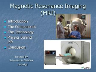
Introduction to MRI (Magnetic Resonance Imaging). Speaker : Tsung-Hsueh Lee Advisor : Prof. Tzi-Dar Chiueh Date : March 21, 2005. Outline. Physic phenomena Spatial Encoding Image Construction Fast scanning MRI Hardware Conclusion Reference. Physic phenomena Spatial Encoding

E N D
Introduction to MRI(Magnetic Resonance Imaging) Speaker:Tsung-Hsueh Lee Advisor:Prof. Tzi-Dar Chiueh Date:March 21, 2005
Outline • Physic phenomena • Spatial Encoding • Image Construction • Fast scanning • MRI Hardware • Conclusion • Reference
Physic phenomena • Spatial Encoding • Image Construction • Fast scanning • MRI Hardware • Conclusion • Reference
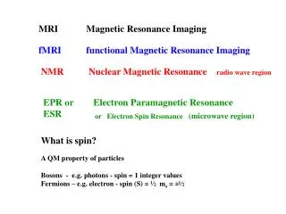
magnetic moment spin Spinning • Spinning charged particle creates an electromagnetic field • Spin quantum number S # of energy states = 2S+1 M=0
Z B0 J or Y |B0|••t X Precession • Larmor Equation • Why hydrogen nucleus • 1. Large component of human body • 2. Odd number of protons (unpaired protons) B0 field
Energy Level • Energy state is not always the same • For 1H B0=1.5T Energy State=2 Precession frequency= 42.58MHz/T*1.5T=64MHz Nuclei Unpaired Protons Unpaired Neutrons Net Spin (MHz/T) 1H 1 0 1/2 42.58 2H 1 1 1 6.54 31P 0 1 1/2 17.25 23Na 0 1 3/2 11.27 14N 1 1 1 3.08 13C 0 1 1/2 10.71 19F 0 1 1/2 40.08
RF Pulse • If the pulse F equals Larmor F Resonance • Rf pulse causes a flip angle and also makes protons get in phase • Some protons will change energy state Ө MXY
900 pulse and 1800 pulse • 900 pulse lets MXY=M0 and • Used to excite protons • Partial flip • 1800 inverts M0 and precession direction
T1 Relaxation Time • After RF pulse • 1. Spins go back to the lowest energy state • 2. Spins get out of phase • T1 also called spin-lattice relaxation time • Spins give energy to the surrounding lattice
M M(t) 0 | | t T 2 T2* Relaxation Time • Due to • Interactions among individual spins • External magnetic field inhomogeneity
T2 and T2* • Use 1800 pulse to refocus • Eliminate the effect of external magnetic field T2 Relaxation Time or spin-spin relaxation time
T1 and T2 • T2 usually much faster than T1
Pulse Sequence • TR - time to repeat 900 pulse • TE – time to echo • Spin Echo (SE) Sequence
Short TR Long TR T1 Weighted Image • Very long TR – T1 effectcanceled • Short TR short TE – T1 weighted image
T2 Weighted Image • Long TE – T2 weighted image • Very short TR – Signal intensity too small
Physic phenomena • Spatial Encoding • Image Construction • Fast scanning • MRI Hardware • Conclusion • Reference
Slice-Select Gradient • Use different RF to excite different slices • Thickness • Frequency range • Gradient B0
Frequency and Phase Encoding • Use Gy gradient to create a phase difference among different rows • Phase shift between each row 360/# of rows • Use Gx gradient when sampling to create different precession F among different columns
Phase Encoding • How does phase encoding work?
Example 1. 2. Gy 3. 4. Gx
Example 1cos(ω1t+00) 0.8cos(ω2t+00) 1 1cos(ω1t+900) 0.8cos(ω2t+1800) 0.8 0.8cos(ω2t+3600) 1cos(ω1t+1800) 1cos(ω1t+2700) 0.8cos(ω2t+5400)
Physic phenomena • Spatial Decoding • Image Construction • Fast scanning • MRI Hardware • Conclusion • Reference
Sample • Nyquist Law
Data Space and K Space • Maximal signal intensity will be in the center • Due to refocusing for each row • Due to different dephasing rate for each column Different Phase Encoding Sample
FT Process • Split signal into two parts, real and imaginary • 1st 1DFT for each row • Modulus • 2nd 1DFT for each column
Another way to construct imaging Select one slice Do many experiments with different directions of readout gradient
Physic phenomena • Spatial Decoding • Image Construction • Fast scanning • Conclusion • Reference
Multi-Slice Imaging • TR much longer than TE • Put different excitation in that time interval
FSE • Fast Spin Echo • Echo Train Length (ETL) • Different TE for different echo • Choose refocus timing at the TE we want
Gx GRE • Gradient Recalled Echo • Why not decrease TR? • Partial flip angle • 1800 pulse can’t be used • Another way to refocus
EPI • Echo Planar Imaging • One shot and Multi-shot • Signal decays rapidly because T2* • FOV (Field of View) too big • Requirement is hard to achieve
Physic phenomena • Spatial Encoding • Image Construction • Fast scanning • MRI Hardware • Conclusion • Reference
B0 Magnet and Gradient Coil 0.015 – 0.3 Tesla Resistive 0.5 – 3 Tesla Superconducting
Conclusion • MRI is a very powerful and complicated system. • There are already many advanced techniques.
Reference • MRI The Basics, Ray H. Hashermi, William G. Bradley • Principlesof Magnetic ResonanceImaging, Zhi-Pei Liang, Paul C. Lauterbur • MRI Physicsfor Radiologist, Alfred L. Horowitz • Fundamentalsof MAGNETICRESONANCE IMAGING, Donald W. Chakeres, PetraSchmalbrock • “MRI madeeasy” program, Schering
Z |B1|••t B0 J or or M Y |B0|••t B1 |B0|••t X
Spin Echo 900 1800 RF slice phase readout echo signal TE
RF pulse Gz Gy GX A B D E C K Space Image Space Coherent detector Complex numbers I + jQ __________________ __________________ DFT __________________ __________________ __________________ __________________ __________________ ‘Real numbers’
Fourier transform af FID F time frequency F-1
Gradient Echopulse timing a0 RF slice phase readout echo signal TE