Download
1 / 37
370 likes | 414 Views
Law of Demand. There is an inverse relationship between the price of a good and the quantity of the good demanded per time period. Substitution Effect Income Effect. Individual Consumer’s Demand Qd X = f(P X , I, P Y , T). Qd X = P X = I = P Y = T =.

E N D
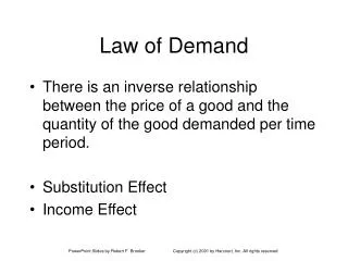
Law of Demand • There is an inverse relationship between the price of a good and the quantity of the good demanded per time period. • Substitution Effect • Income Effect
Individual Consumer’s DemandQdX = f(PX, I, PY, T) QdX = PX = I = PY = T = quantity demanded of commodity X by an individual per time period price per unit of commodity X consumer’s income price of related (substitute or complementary) commodity tastes of the consumer
QdX = f(PX, I, PY, T) QdX/PX < 0 QdX/I > 0 if a good is normal QdX/I < 0 if a good is inferior QdX/PY > 0 if X and Y are substitutes QdX/PY < 0 if X and Y are complements
Market Demand Curve • Horizontal summation of demand curves of individual consumers • Bandwagon Effect • Snob Effect
Market Demand FunctionQDX = f(PX, N, I, PY, T) QDX = PX = N = I = PY = T = quantity demanded of commodity X price per unit of commodity X number of consumers on the market consumer income price of related (substitute or complementary) commodity consumer tastes
Demand Faced by a Firm • Market Structure • Monopoly • Oligopoly • Monopolistic Competition • Perfect Competition • Type of Good • Durable Goods • Nondurable Goods • Producers’ Goods - Derived Demand
Linear Demand Function QX = a0 + a1PX + a2N + a3I + a4PY + a5T PX Intercept:a0 + a2N + a3I + a4PY + a5T Slope:QX/PX = a1 QX
Price Elasticity of Demand Point Definition Linear Function
Price Elasticity of Demand Arc Definition
Expressing Economic Relationships Equations: TR = 100Q - 10Q2 Tables: Graphs:
Concept of the Derivative The derivative of Y with respect to X is equal to the limit of the ratio Y/X as X approaches zero.
Rules of Differentiation Constant Function Rule: The derivative of a constant, Y = f(X) = a, is zero for all values of a (the constant).
Rules of Differentiation Power Function Rule: The derivative of a power function, where a and b are constants, is defined as follows.
Rules of Differentiation Sum-and-Differences Rule: The derivative of the sum or difference of two functions U and V, is defined as follows.
Rules of Differentiation Product Rule: The derivative of the product of two functions U and V, is defined as follows.
Rules of Differentiation Quotient Rule: The derivative of the ratio of two functions U and V, is defined as follows.
Rules of Differentiation Chain Rule: The derivative of a function that is a function of X is defined as follows.
Optimization With Calculus Find X such that dY/dX = 0 Second derivative rules: If d2Y/dX2 > 0, then X is a minimum. If d2Y/dX2 < 0, then X is a maximum.
MR>0 MR<0 MR=0 Marginal Revenue, Total Revenue, and Price Elasticity TR QX
Determinants of Price Elasticity of Demand Demand for a commodity will be more elastic if: • It has many close substitutes • It is narrowly defined • More time is available to adjust to a price change
Determinants of Price Elasticity of Demand Demand for a commodity will be less elastic if: • It has few substitutes • It is broadly defined • Less time is available to adjust to a price change
Income Elasticity of Demand Point Definition Linear Function
Income Elasticity of Demand Arc Definition Normal Good Inferior Good
Cross-Price Elasticity of Demand Point Definition Linear Function
Cross-Price Elasticity of Demand Arc Definition Substitutes Complements
Other Factors Related to Demand Theory • International Convergence of Tastes • Globalization of Markets • Influence of International Preferences on Market Demand • Growth of Electronic Commerce • Cost of Sales • Supply Chains and Logistics • Customer Relationship Management
Cost-Volume-Profit Analysis Total Revenue = TR = (P)(Q) Total Cost = TC = TFC + (AVC)(Q) Breakeven Volume TR = TC (P)(Q) = TFC + (AVC)(Q) QBE = TFC/(P - AVC)
Cost-Volume-Profit Analysis P = 40 TFC = 200 AVC = 5 QBE = 40
Operating Leverage Operating Leverage = TFC/TVC Degree of Operating Leverage = DOL
Operating Leverage TC’ has a higher DOL than TC and therefore a higher QBE
BEQ = 40,000 • MOS = 100% • PROFIT = (20-15)X(80000-40000) = 2,00,000 • TARGET PROFIT 5,00,000 requires additional profit of 3,00,000 • Required additional sales quantity is (3,00,000)/(20-15) = 60,000 units • Total sales quantity required for target profit is 1,40,000 units
New Scenario: P – AVC = 18 – 14 = 4 • NEW BEQ = 2,00,000/4 = 50,000 • NEW SALES QUANTITY = 80,000*1.1 = 88,000 • QUANTITY SOLD BEYOND BEQ = 38,000 • PROFIT = 38,000X4 = 1,52,000/-