Download

1 / 55
560 likes | 599 Views
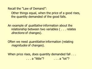
1. 2. Law of Demand. Holding all other things constant ( ceteris paribus ), there is an inverse relationship between the price of a good and the quantity of the good demanded per time period. Substitution Effect Income Effect. Components of Demand: The Substitution Effect.

E N D
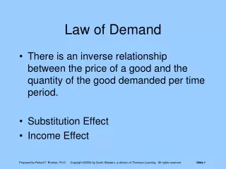
Law of Demand • Holding all other things constant (ceteris paribus), there is an inverse relationship between the price of a good and the quantity of the good demanded per time period. • Substitution Effect • Income Effect
Components of Demand:The Substitution Effect • Assuming that real income is constant: • If the relative price of a good rises, then consumers will try to substitute away from the good. Less will be purchased. • If the relative price of a good falls, then consumers will try to substitute away from other goods. More will be purchased. • The substitution effect is consistent with the law of demand.
Components of Demand:The Income Effect • The real value of income is inversely related to the prices of goods. • A change in the real value of income: • will have a direct effect on quantity demanded if a good is normal. • will have an inverse effect on quantity demanded if a good is inferior. • The income effect is consistent with the law of demand only if a good is normal.
Individual Consumer’s DemandQdX = f(PX, I, PY, T) QdX = PX = I = PY = T = quantity demanded of commodity X by an individual per time period price per unit of commodity X consumer’s income price of related (substitute or complementary) commodity tastes of the consumer
QdX = f(PX, I, PY, T) QdX/PX < 0 QdX/I > 0 if a good is normal QdX/I < 0 if a good is inferior QdX/PY > 0 if X and Y are substitutes QdX/PY < 0 if X and Y are complements
Market Demand Curve • Horizontal summation of demand curves of individual consumers • Exceptions to the summation rules • Bandwagon Effect • collective demand causes individual demand • Snob (Veblen) Effect • conspicuous consumption • a product that is expensive, elite, or in short supply is more desirable
Market Demand FunctionQDX = f(PX, N, I, PY, T) QDX = PX = N = I = PY = T = quantity demanded of commodity X price per unit of commodity X number of consumers on the market consumer income price of related (substitute or complementary) commodity consumer tastes
Demand Curve Faced by a Firm Depends on Market Structure • Market demand curve • Imperfect competition • Firm’s demand curve has a negative slope • Monopoly - same as market demand • Oligopoly • Monopolistic Competition • Perfect Competition • Firm is a price taker • Firm’s demand curve is horizontal
Demand Curve Faced by a Firm Depends on the Type of Product • Durable Goods • Provide a stream of services over time • Demand is volatile • Nondurable Goods and Services • Producers’ Goods • Used in the production of other goods • Demand is derived from demand for final goods or services
Linear Demand Function QX = a0 + a1PX + a2N + a3I + a4PY + a5T PX Intercept:a0 + a2N + a3I + a4PY + a5T Slope:QX/PX = a1 QX
Linear Demand Function Example Part 1 Demand Function for Good X QX = 160 - 10PX + 2N + 0.5I + 2PY + T Demand Curve for Good X Given N = 58, I = 36, PY = 12, T = 112 Q = 430 - 10P
Linear Demand Function Example Part 2 Inverse Demand Curve P = 43 – 0.1Q Total and Marginal Revenue Functions TR = 43Q – 0.1Q2 MR = 43 – 0.2Q
Price Elasticity of Demand Point Definition Linear Function
Price Elasticity of Demand Arc Definition
MR>0 MR<0 MR=0 Marginal Revenue, Total Revenue, and Price Elasticity TR QX
Determinants of Price Elasticity of Demand The demand for a commodity will be more price elastic if: • It has more close substitutes • It is more narrowly defined • More time is available for buyers to adjust to a price change
Determinants of Price Elasticity of Demand The demand for a commodity will be less price elastic if: • It has fewer substitutes • It is more broadly defined • Less time is available for buyers to adjust to a price change
Income Elasticity of Demand Point Definition Linear Function
Income Elasticity of Demand Arc Definition Normal Good Inferior Good
Cross-Price Elasticity of Demand Point Definition Linear Function
Cross-Price Elasticity of Demand Arc Definition Substitutes Complements
Example: Using Elasticities inManagerial Decision Making A firm with the demand function defined below expects a 5% increase in income (M) during the coming year. If the firm cannot change its rate of production, what price should it charge? • Demand: Q = – 3P + 100M • P = Current Real Price = 1,000 • M = Current Income = 40
Solution • Elasticities • Q = Current rate of production = 1,000 • P = Price = - 3(1,000/1,000) = - 3 • I = Income = 100(40/1,000) = 4 • Price • %ΔQ = - 3%ΔP + 4%ΔI • 0 = -3%ΔP+ (4)(5) so %ΔP = 20/3 = 6.67% • P = (1 + 0.0667)(1,000) = 1,066.67
Other Factors Related to Demand Theory • International Convergence of Tastes • Globalization of Markets • Influence of International Preferences on Market Demand • Growth of Electronic Commerce • Cost of Sales • Supply Chains and Logistics • Customer Relationship Management
Indifference Curves • Utility Function: U = U(QX,QY) • Marginal Utility > 0 • MUX = ∂U/∂QX and MUY = ∂U/∂QY • Second Derivatives • ∂MUX/∂QX < 0 and ∂MUY/∂QY < 0 • ∂MUX/∂QY and ∂MUY/∂QX • Positive for complements • Negative for substitutes
Marginal Rate of Substitution • Rate at which one good can be substituted for another while holding utility constant • Slope of an indifference curve • dQY/dQX = -MUX/MUY
QY QY QX QX Indifference Curves:Complements and Substitutes Perfect Complements Perfect Substitutes
The Budget Line • Budget = M = PXQX + PYQY • Slope of the budget line • QY = M/PY - (PX/PY)QX • dQY/dQX = - PX/PY
Budget Lines: Change in Price GF: M = $6, PX = PY = $1 GF’: PX = $2 GF’’: PX = $0.67
Budget Lines: Change in Income GF: M = $6, PX = PY = $1 GF’: M = $3, PX = PY = $1