Download
1 / 34
340 likes | 514 Views
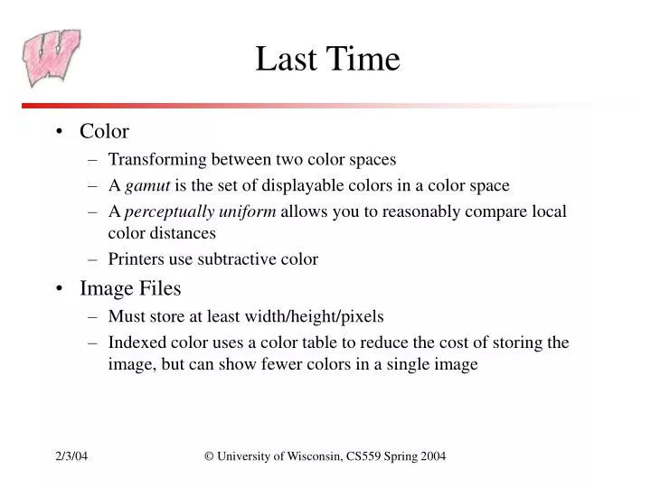
Last Time. Color Transforming between two color spaces A gamut is the set of displayable colors in a color space A perceptually uniform allows you to reasonably compare local color distances Printers use subtractive color Image Files Must store at least width/height/pixels

E N D
Last Time • Color • Transforming between two color spaces • A gamut is the set of displayable colors in a color space • A perceptually uniform allows you to reasonably compare local color distances • Printers use subtractive color • Image Files • Must store at least width/height/pixels • Indexed color uses a color table to reduce the cost of storing the image, but can show fewer colors in a single image © University of Wisconsin, CS559 Spring 2004
Today • JPEG images • Color quantization • Dithering • Homework 1 due, here, now © University of Wisconsin, CS559 Spring 2004
JPEG • Multi-stage process intended to get very high compression with controllable quality degradation • Start with YIQ color • Why? Recall, it’s the color standard for TV © University of Wisconsin, CS559 Spring 2004
A transformation to convert from the spatial to frequency domain – done on 8x8 blocks Why? Humans have varying sensitivity to different frequencies, so it is safe to throw some of them away Basis functions: Each block of 8x8 pixels is a linear combination of these images Discrete Cosine Transform © University of Wisconsin, CS559 Spring 2004
Quantization • Reduce the number of bits used to store each coefficient by dividing by a given value • If you have an 8 bit number (0-255) and divide it by 8, you get a number between 0-31 (5 bits = 8 bits – 3 bits) • Different coefficients are divided by different amounts • Perceptual issues come in here • Achieves the greatest compression, but also quality loss • “Quality” knob controls how much quantization is done © University of Wisconsin, CS559 Spring 2004
Entropy Coding • Standard lossless compression on quantized coefficients • Delta encode the DC components • Run length encode the AC components • Lots of zeros, so store number of zeros then next value • Huffman code the encodings © University of Wisconsin, CS559 Spring 2004
Lossless JPEG With Prediction • Predict what the value of the pixel will be based on neighbors • Record error from prediction • Mostly error will be near zero • Huffman encode the error stream • Works really well for fax messages © University of Wisconsin, CS559 Spring 2004
Color Quantization • The problem of reducing the number of colors in an image with minimal impact on appearance • Extreme case: 24 bit color to black and white • Less extreme: 24 bit color to 256 colors, or 256 grays • Why do we care? • Sub problems: • Decide which colors to use in the output (if there is a choice) • Decide which of those colors should be used for each input pixel © University of Wisconsin, CS559 Spring 2004
Example (24 bit color) © University of Wisconsin, CS559 Spring 2004
Uniform Quantization • Break the color space into uniform cells • Find the cell that each color is in, and map it to the center • Generally does poorly because it fails to capture the distribution of colors • Some cells may be empty, and are wasted • Equivalent to dividing each color by some number and taking the integer part • Say your original image is 24 bits color (8 red, 8 green, 8 blue) • Say you have 256 colors available, and you choose to use 8 reds, 8 greens and 4 blues (8 × 8 × 4 = 256 ) • Divide original red by 32, green by 32, and blue by 64 • Some annoying details © University of Wisconsin, CS559 Spring 2004
Uniform Quantization • 8 bits per pixel in this image • Note that it does very poorly on smooth gradients • Normally the hardest part to get right, because lots of similar colors appear very close together • Does this scheme use information from the image? © University of Wisconsin, CS559 Spring 2004
Populosity Algorithm • Build a color histogram: count the number of times each color appears • Choose the n most commonly occurring colors • Typically group colors into small cells first using uniform quantization • Map other colors to the closest chosen color • Problem? © University of Wisconsin, CS559 Spring 2004
Populosity Algorithm • 8 bit image, so the most popular 256 colors • Note that blue wasn’t very popular, so the crystal ball is now the same color as the floor • Populosity ignores rare but important colors! © University of Wisconsin, CS559 Spring 2004
Median Cut (Clustering) • View the problem as a clustering problem • Find groups of colors that are similar (a cluster) • Replace each input color with one representative of its cluster • Many algorithms for clustering • Median Cut is one: recursively • Find the “longest” dimension (r, g, b are dimensions) • Choose the median of the long dimension as a color to use • Split into two sub-clusters along the median plane, and recurse on both halves • Works very well in practice © University of Wisconsin, CS559 Spring 2004
Median Cut • 8 bit image, so 256 colors • Now we get the blue • Median cut works so well because it divides up the color space in the “most useful” way © University of Wisconsin, CS559 Spring 2004
Optimization Algorithms • The quantization problem can be phrased as optimization • Find the set of colors and mapping that result in the lowest quantization error • Several methods to solve the problem, but of limited use unless the number of colors to be chosen is small • It’s expensive to compute the optimum • It’s also a poorly behaved optimization © University of Wisconsin, CS559 Spring 2004
Perceptual Problems • While a good quantization may get close colors, humans still perceive the quantization • Biggest problem: Mach bands • The difference between two colors is more pronounced when they are side by side and the boundary is smooth • This emphasizes boundaries between colors, even if the color difference is small • Rough boundaries are “averaged” by our vision system to give smooth variation © University of Wisconsin, CS559 Spring 2004
Mach Bands in Reality The floor appears banded © University of Wisconsin, CS559 Spring 2004
Mach Bands in Reality Still some banding even in this 24 bit image (the floor in the background) © University of Wisconsin, CS559 Spring 2004
Mach bands Emphasized • Note that each bar on the left appears to have color variation across it • Left edge appears darker than right • The effect is entirely due to Mach banding © University of Wisconsin, CS559 Spring 2004
Dithering (Digital Halftoning) • Mach bands can be removed by adding noise along the boundary lines • General perceptive principle: replaced structured errors with noisy ones and people complain less • Old industry dating to the late 1800’s • Methods for producing grayscale images in newspapers and books © University of Wisconsin, CS559 Spring 2004
Dithering to Black-and-White • Black-and-white is still the preferred way of displaying images in many areas • Black ink is cheaper than color • Printing with black ink is simpler and hence cheaper • Paper for black inks is not special • To get color to black and white, first turn into grayscale: I=0.299R+0.587G+0.114B • This formula reflects the fact that green is more representative of perceived brightness than blue is • NOTE that it is not the equation implied by the RGB->XYZ color space conversion matrix © University of Wisconsin, CS559 Spring 2004
Sample Images © University of Wisconsin, CS559 Spring 2004
Threshold Dithering • For every pixel: If the intensity < 0.5, replace with black, else replace with white • 0.5 is the threshold • This is the naïve version of the algorithm • To keep the overall image brightness the same, you should: • Compute the average intensity over the image • Use a threshold that gives that average • For example, if the average intensity is 0.6, use a threshold that is higher than 40% of the pixels, and lower than the remaining 60% • For all dithering we will assume that the image is gray and that intensities are represented as a value in [0, 1.0] • If you have a 0-255 image, you can scale all the thresholds (multiply by 255) © University of Wisconsin, CS559 Spring 2004
Naïve Threshold Algorithm © University of Wisconsin, CS559 Spring 2004
Random Modulation • Add a random amount to each pixel before thresholding • Typically add uniformly random amount from [-a,a] • Pure addition of noise to the image • For better results, add better quality noise • For instance, use Gaussian noise (random values sampled from a normal distribution) • Should use same procedure as before for choosing threshold • Not good for black and white, but OK for more colors • Add a small random color to each pixel before finding the closest color in the table © University of Wisconsin, CS559 Spring 2004
Random Modulation © University of Wisconsin, CS559 Spring 2004
Ordered Dithering • Break the image into small blocks • Define a threshold matrix • Use a different threshold for each pixel of the block • Compare each pixel to its own threshold • The thresholds can be clustered, which looks like newsprint • The thresholds can be “random” which looks better Threshold matrix © University of Wisconsin, CS559 Spring 2004
Clustered Dithering 22 23 10 20 14 25 3 8 5 17 15 6 1 2 11 12 9 4 7 21 18 19 13 24 16 © University of Wisconsin, CS559 Spring 2004
Dot Dispersion 2 16 3 13 10 6 11 7 4 14 1 15 12 8 9 5 © University of Wisconsin, CS559 Spring 2004
Pattern Dithering • Compute the intensity of each sub-block and index a pattern • NOT the same as before • Here, each sub-block has one of a fixed number of patterns – pixel is determined only by average intensity of sub-block • In ordered dithering, each pixel is checked against the dithering matrix before being turned on © University of Wisconsin, CS559 Spring 2004
Floyd-Steinberg Dithering • Start at one corner and work through image pixel by pixel • Usually scan top to bottom in a zig-zag • Threshold each pixel • Compute the error at that pixel: The difference between what should be there and what you did put there • Propagate error to neighbors by adding some proportion of the error to each unprocessed neighbor • Mask tells you how much to add e 7/16 3/16 5/16 1/16 © University of Wisconsin, CS559 Spring 2004
Floyd-Steinberg Dithering © University of Wisconsin, CS559 Spring 2004
Color Dithering • All the same techniques can be applied, with some modification • Below is Floyd-Steinberg: Error is difference from nearest color in the color table, error propagation is the same © University of Wisconsin, CS559 Spring 2004