Download
1 / 16
160 likes | 263 Views
Chapter 22: Aggregate Supply Analysis. Aggregate Supply Curve – relationship between the quantity of output supplied and the inflation rate. If prices and wages take time to adjust to their long-run level, the aggregate supply curve differs in the short run and long run.

E N D
Chapter 22: Aggregate Supply Analysis Aggregate Supply Curve – relationship between the quantity of output supplied and the inflation rate. If prices and wages take time to adjust to their long-run level, the aggregate supply curve differs in the short run and long run. Long Run Aggregate Supply Curve (LRAS) – denotes the amount of output that can be produced by the economy in the long run (Potential Output). Potential output is determined by: • Amount of capital in the economy • Total amount of labor supplied at full employment • Available technology that puts labor and capital together to produce goods and services, G/S. Natural Rate of Output (Potential Output) is the level of output produced at the Natural Rate of Unemployment (where the unemployment rate gravitates to in the long run). This is where the economy settles in the long-run for any inflation rate, DP/P.
AD/AS Model PL LRAS1 LRAS2 Y Y1Pot Y2Pot In the LR, YPot = f( # of workers K stock Technology) not PL L1FE L2FE PF2 PF1 Labor
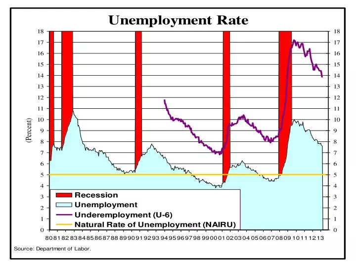
Shifts in LRAS Shifts in Long Run Aggregate Supply (LRAS) Curve A. The 3 factors listed below grow fairly steadily over time, so potential output increases over time. To simplify matters, when YP is growing steadily over time we represent YP as fixed. • Amount of capital in the economy • Total amount of labor supplied at full employment • Available technology that puts labor and capital together to produce G/S. B. D in the Natural Rate of Unemployment If Natural Rate of Unemployment falls (ex. 4.5%) (labor is more heavily utilized) => YP If Natural Rate of Unemployment rises (ex. 6%) (due to retiring baby boomers) => YP (slows down the natural rate of output growth, 3% to 2.5%)
Short Run Aggregate Supply Curve DP/P = (DP/P)et+1 + g [Y – YP] – r where (DP/P)et+1 = Expected future inflation. Inflation, DP/P, will rise one-for-one with increase in (DP/P)et+1. Workers and firms care about real wages (w/P = x = amount of G/S wages can buy). If workers expect higher inflation in the future, they will demand higher wages to maintain real wages. Because labor costs typically makeup 70% of a firms costs, businesses will increase prices to maintain profit margins. [Y – YP] = output gap is the difference between aggregate output and potential output. g = sensitivity of DP/P to the output gap. g > 0 creating an upward sloping SRAS curve. If [Y – YP] > 0, then there is little slack in the economy, labor markets get tight, workers demand higher wages, and firms take opportunity to increase prices => higher DP/P If [Y – YP] < 0, then there is lots of slack in the economy, workers accept smaller increases in wages, and firms need to lower prices to sell their goods => lower DP/P r = Price (Supply) Shocks – occur when there is a shock to the supply of G/S produced in the economy. Examples: Oil supply restrictions, developing countries rising demand for commodities, a falling exchange rate pushing up import prices, workers pushing for wage gains higher than productivity gains (Cost-push Inflation).
Short Run Aggregate Supply Curve DP/P = (DP/P)et+1 + g [Y – YP] – r SRAS curve implies that wages and prices are sticky in the short-run (the aggregate price level adjusts slowly over time). The more flexible wages and prices are, the more DP/P responds to deviations of output, Y, from potential output, YP. This will increase the absolute value of g and create a steeper curve. If wages and prices are completely flexible, then g gets very large and the SRAS = LRAS. Shifts in SRAS (DP/P)et+1 . (shifts curve up and to the left) Supply shock, r. (shifts curve up and to the left) Persistent output gap, [Y – YP] => D (DP/P)et+1 . If [Y – YP] > 0 is persistent, then the rise in DP/P due to the movement along the SRAS curve, (g [Y – YP]) => (DP/P)et+1 which shifts the SRAS curve up and back. When [Y – YP] = 0 , then the SRAS stops shifting up because DP/P and (DP/P)et+1 stop rising. If [Y – YP] < 0 is persistent, then the fall in DP/P due to the movement along the SRAS curve, (g [Y – YP]) => (DP/P)et+1 which shifts the SRAS curve down and to the right. Shifting stops when Y = YP
General Equilibrium in the AD & AS Analysis All markets are simultaneously in equilibrium – Quantity of aggregate output demanded is equal to quantity of aggregate output supplied. Self-Correcting Mechanism – over time the short-run equilibrium moves/migrates to the long-run equilibrium. So if Y* = YP ,the short-run equilibrium, Y* will move over time to reach YP. If the current level of DP/P changes from its initial level, the SRAS curve will shift as wages and prices adjust to a new DP/P)et+1. This shift over time will restore the economy to long-run equilibrium at full employment and YP.
Econ 330 Chapter 22 HomeworkDue Friday, May 2 Chapter 22 Questions & Applied Problems 8, 11, 13, 14, 21, 23, 24