Download
1 / 9
90 likes | 165 Views
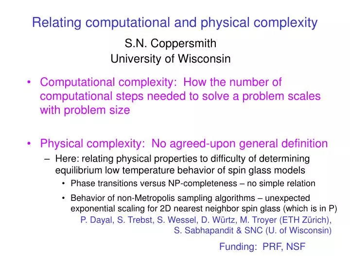
Relating computational and physical complexity. S.N. Coppersmith University of Wisconsin. Computational complexity: How the number of computational steps needed to solve a problem scales with problem size Physical complexity: No agreed-upon general definition

E N D
Relating computational and physical complexity S.N. Coppersmith University of Wisconsin • Computational complexity: How the number of computational steps needed to solve a problem scales with problem size • Physical complexity: No agreed-upon general definition • Here: relating physical properties to difficulty of determining equilibrium low temperature behavior of spin glass models • Phase transitions versus NP-completeness – no simple relation • Behavior of non-Metropolis sampling algorithms – unexpected exponential scaling for 2D nearest neighbor spin glass (which is in P) P. Dayal, S. Trebst, S. Wessel, D. Würtz, M. Troyer (ETH Zürich), S. Sabhapandit & SNC (U. of Wisconsin) Funding: PRF, NSF
Ferromagnetic bond Antiferromagnetic bond ? Spin glass (Edwards-Anderson, 1975) Pairs of spins coupled by both ferromagnetic and antiferromagnetic bonds Competing interactions frustration (many different configurations with same energy)
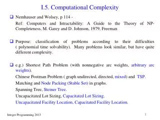
For nearest neighbor spin glass, no simple relation between computational complexity and presence of physical phase transition • 3D: Finding ground state is NP-complete (Barahona ‘82), model has phase transition at nonzero temperature T • 2D, single layer: finding ground state is in P (Bieche et al., 1980), no phase transition at nonzero T • 2D, two-layer: finding ground state is NP-complete (Barahona ’82), no phase transition
Characterizing algorithms for determining statistical mechanical properties of spin glass models • Monte Carlo (weight configurations by e-(energy/temperature)) Expect logarithmically slow relaxation for spin glass in any dimension (because of energy barriers between low-lying exciting states and ground state) (Huse and Fisher (PRL 57, 2203 (1986)) • Flat histogram methods (weight configurations by 1/(density of states)) Can overcome free energy barriers get apparent polynomial scaling for frustrated Ising model, but not for 2-D spin glass
Flat histogram methods for overcoming tunneling barriers between local free energy minima (multicanonical method, parallel tempering, Wang-Landau sampling) Usual Monte Carlo: weight configuration by exp(energy/temperature) Flat histogram: weight configuration by 1/(density of states) equally likely to move up and down in energy log (density of states) energy # of configurations accepted energy Flat histogram algorithms generate density of states in course of calculation; we obtain general limits by examining performance using exact density of states as weighting function (for certain models).
Characterize algorithm speed using tunneling time (time to sample energy range) Tunneling time scales as power of system size for ferromagnetic Ising model and for fully frustrated Ising model (though not simple random walk in energy)
For 2-D J spin glass, tunneling times are broadly distributed (Fréchet distribution), and appear to scale exponentially with system size Probability Fréchet cumulative probability distribution (<0)
Correlation between tunneling times and properties of energy surface
Relationship between computational complexity and physical complexity is nontrivial Flat histogram algorithms have faster performance than usual Monte Carlo, but slower than “expected” Summary Questions • What determines scaling of flat histogram algorithms? • What are relationships between algorithms and physical processes?