Download
1 / 33
330 likes | 425 Views
I.5. Computational Complexity. Nemhauser and Wolsey, p 114 - Ref: Computers and Intractability: A Guide to the Theory of NP-Completeness, M. Garey and D. Johnson, 1979, Freeman

E N D
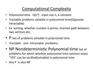
I.5. Computational Complexity • Nemhauser and Wolsey, p 114 - Ref: Computers and Intractability: A Guide to the Theory of NP-Completeness, M. Garey and D. Johnson, 1979, Freeman • Purpose: classification of problems according to their difficulties ( polynomial time solvability). Many problems look similar, but have quite different complexity. • e.g.) Shortest Path Problem (with nonnegative arc weights, arbitrary arc weights). Chinese Postman Problem ( graph undirected, directed, mixed) and TSP. Matching and Node Packing (Stable Set) in graphs. Spanning Tree, Steiner Tree. Uncapacitated Lot Sizing, Capacitated Lot Sizing. Uncapacitated Facility Location, Capacitated Facility Location.
Mixed integer programming problem max LP, IP are special cases of MIP, hence MIP is at least as hard as IP and LP. • See Fig 1.1 (P116, NW) for classification of problems Note that the problems in the figure may have a little bit different meaning from earlier definitions. • Observations If MIP easy, then LP, IP easy If LP and/or IP hard, then MIP hard If MIP hard, but LP and/or IP may be easy.
2.Measuring alg efficiency and prob complexity • Def: problem instance: specified by assigning data to problem parameters size of a problem: length of information to represent the problem in binary alphabet. ( and positive integer, then represent rational number by two integers, incidence (characteristic) vectors for sets, node-edge incidence matrix, adjacency matrix for graphs, Only compact representation acceptable, e. g. TSP )
Running time of algorithm : • Arithmetic model: assume each instruction takes unit time • Bit model: each instruction on single bit takes unit time Use a simple majorizing function to represent the asymptotic behavior of the running time with respect to the size of the problem. Worst-case view point. • Advantage: 1. absolute guarantee 2. Make no assumption on distribution of data 3. easier to analyze Disadvantage: very conservative estimate (e.g. simplex method for LP) • Algorithm is said to be polynomial time algorithm if for some fixed .
Note • Size of data must be considered ( dynamic programming algorithm for knapsack problem is not polynomial time algorithm since which is not polynomial in . ) (unary encoding not allowed) • Size of the numbers during computation must remain polynomially bounded of the input data ( ) ( length of the encoding of the numbers must remain polynomial of , e.g. ellipsoid method for LP needs to compute square root. ) • Def:P is the class of problems that can be solved in polynomial time ( more precisely, the feasibility problem form of the problem )
3. Some Problems Solvable in Polynomial Time • Problems in P • Shortest path problem with nonnegative edge weights • Solving linear equations • Transportation problem ( using scaling of data, polynomial in ) (For general network flow problem, Tardos found strongly polynomial time algorithm (algorithm such that the running time is polynomial in problem parameter (e.g. ), but independent of data size ) • The linear programming problem ( ellipsoid method, interior point methods )
Certificate of optimality Information that can be used to check optimality of a solution in polynomial time. (length of the encoding of information must be polynomially bounded of the length of the input.) • Problem in certificate of optimality ( problem itself, use the poly time algorithm to verify the optimality) certificate of optimality (likely that) problem is in
LP : , Then certificate of optimality for LP is primal, dual basic feasible solution. Size of certificate is polynomially bounded? • Prop 3.1:: extreme point and extreme ray of integral, A is . Then, for i) ii) Pf) (i) extreme point of is a solution of where is and nonsingular. From Cramer’s rule, ( determinant of det of matrix obtained by replacing th column of by ). Number of terms in det is ( ), hence and (ii) is determined by equations. ( or )
Number of digits to represent ~ polynomial function of log . short proof • Above result indicates that we can solve any LP as problem on polytope ( used in ellipsoid algorithm for LP )
Certificate of optimality for matching problem (IP problem) : with nodes and edges max for add odd set constraints: for all and odd extreme points of LP relaxation are incidence vectors of matchings. But can’t use polynomial solvability of LP directly (number of constraints exponential in the size of data) • However, certificate of optimality exists. Choose constraints that correspond to positive dual variables in optimal solution. (basic dual solution has no more than positive variables) Note that we do not need to check the odd set constraints for violation once a matching solution is given.
4. Remarks on 0-1 and Pure-Integer Prog. • Consider the running time for IP (brute force enumeration) and bounds on the size of solutions. • 0-1 integer: total enumeration takes some subclass solvable in polynomial time • Integer knapsack : dynamic programming algorithm. • Pure integer: Let P bounded total enumeration P unbounded?
Thm 4.1: extreme point of conv(), , then Pf) From Thm 6.1, 6.2 of section I.4.6 (p104), , where for and . ( integer for ( ) Any extreme point of conv() must be one of the points , that is, any extreme point , , where are extreme points and are extreme rays of P. Since and hence
Note that where Let can give bounds enumeration • Technique to transform general IP to 0-1 IP Let binary, length polynomially bounded ( objective coeff: max • Complexity of algorithm (enumeration) for IP : Integer Programming with fixed • 0-1 IP P (enumeration algorithm) • For general IP, enumeration is not polynomial even for fixed n. (depends on data size) ( not polynomial even fixed. transformation to 0-1 IP : one variable variables enumeration is at least polynomial in ( not in ) enumeration not polynomial even for fixed.
However, there exists a theorem that says IP with fixed is in ( using basis reduction algorithm for integer lattices, section I. 7. 5., II. 6. 5. ) ( It says complexity not depend on , but result itself does not have much meaning in terms of practical algorithms.) • Thm 4.3: Suppose where is an integral matrix. If defines a facet of conv(), then the length of the description of the coefficients of is bounded by a polynomial function of and .
5. Nondeterministic Polynomial-Time Algorithms and NP Problems • (Feasibility problem) : set of 0-1 strings (instances of ) : set of feasible instances ( ) ( also called decision problem, language recognition problem by Turing machine) ( algorithm deterministic Turing machine ) Given a is ?
0-1 integer programming feasibility: is the set of all integer matrices • 0-1 integer programming lower bound feasibility: ( note that lower bound feasibility is nontrivial even for ) • Prop 5.1: If 0-1 IP lower bound feasibility problem can be solved in polynomial time, then the 0-1 IP optimization problem can be solved in polynomial time ( by bisection search)
Equivalence of Optimization and Feasibility Problem • Consider 0-1 IP optimization and 0-1 IP lower bound feasibility. Opt : Find max Feas : that satisfies and ? If we can solve Opt easily, then we can use the algorithm for Opt to solve Feas. Hence Opt is at least as hard as Feas. (Feas is no harder than Opt.) Our main purpose is to show that Opt is difficult to solve, so if we can show that Feas is hard, it automatically means that Opt is hard. • It can be shown that Feas is at least as hard as Opt, i. e. if we can solve Feaseasily, we can solve Opt easily. Therefore, Opt and Feas have the same difficulty in terms of polynomial time solvability. These relationship holds for almost all optimization and feasibility problem pairs.
Optimization problem can be further divided into (i) finding optimal value and (ii) finding optimal solution. Suppose we can solve Feas in polynomial time, then by using bisection (binary) search, can find optimal value of Opt efficiently (in iterations, which is polynomial of the input length, assuming length of encoding of is poly of input length). Once we know the optimal value of Opt, we can construct an optimal solution using Feas as subroutine. We fix the value of in Opt as 0 and 1, and ask Feas algorithm which case provides optimal value. Then we can determine the value of x1 in an optimal solution. Repeat the procedure for remaining variables. Total computation is polynomial as long as Feas can be solved in polynomial time. (See GJ p 116-117 for TSP problems, later) • Hence, efficient algorithm for Opt efficient algorithm for Feas
Turing Machine Model • Deterministic Turing Machine : mathematical model of algorithm (refer GJ p.23 - ) Finite State Control Read-write head Tape …. …. 1 -2 -1 2 3 0 -3 4 (Deterministic one-tape Turing machine)
A program for DTM specifies the following information: • A finite set of tape symbols, including a subset of input symbols and a distinguished blank symbol • A finite set of states (start statehalt states and ) • A transition function • Input to a DTM is a string . DTM halts if in or state. • We say DTM program M accepts input iff halts in state when applied to input .
Example , • This DTM program accepts 0-1 strings with rightmost two symbols are zeroes. ( check with 10100 ), i. e. it solves the problem of integer divisibility by 4.)
The language (subset of ) LMrecognized by a DTM program M is given by • We say a DTM program solves the decision problem (feasibility problem) if halts for all input strings over its input alphabet and ‘yes’ instances of the decision problems.
Note that ( * ) instances (‘no’ instances and garbage strings) also can be identified since the DTM always stops, so DTM has capability of solving the decision problem (algorithmically). • Though simple, DTM has all capability (but slowly) that we can do on a computer using algorithm. There are other complicated models of computation, but the capability is the same as one tape DTM (capability of identifying ‘yes’, ‘no’ answer, the speed may be different.) • { : there is a polynomial time DTM program for which }
Certificate of Feasibility, the Class NP, and Nondeterministic Algorithms • Nondeterministic Turing Machine model Finite State Control Guessing Module Guessing head Read-write head Tape …. …. 1 -2 -1 2 3 0 -3 4 (Nondeterministic one-tape Turing machine)
Computation of NDTM consists of two stages (1) guessing stage: Starting from tape square , write some symbol on the tape and move left until the stage stops (2) checking stage: Started when the guessing module activate the finite state control in state . Works the same as DTM. Accepting computation if it halts in state . All other computations ( halting in state or not halt) are non-accepting computations. • Some others define NDTM as having many alternative choices in the transition function . NDTM has the capability(non-determinism) to select the right choice if it leads to accepting state. (DTM is a special case of NDTM) • The language recognized by NDTM program is there is a polynomial time NDTM program for which
In the text (NW), certificate of feasibility () : information that can be used to check the feasibility of a given instance of feasibility problem in polynomial time. Nondeterministic algorithm : Given an instance (1) guessing stage : guess a structure ( binary string) (2) checking stage : algorithm to check 1. If there exists that guessing stage provides, hence output ‘yes’ 2. If no certificate exists, no output (NDTM may give ‘no’ or may not halt (runs forever))
: the class of feasibility problems such that for each instance of the answer is obtained in polynomial time by some nondeterministic algorithm. ( nothing is said when ) ( may stand for Nondeterministic Polynomial time) • Note that the symmetry between answers ‘yes’ and ‘no’ for the problems in P may not hold for problems in . For problems in P, ‘no’ answer can be obtained in poly time (for ) since the DTM always halts in poly time on a given instance. (Just exchange ‘yes’, ‘no’ answers. Consider shortest path case) But, for problems in , ‘no’ answer may not be obtained in poly time even by NDTM. (Consider TSP problem). However, ‘no’ answer may be obtained in exponential time by NDTM (or DTM).
Ex: 0-1 integer feasibility is in guessing stage : guess an checking stage : If then General integer feasibility is in use Theorem 4.1 Hamiltonian cycle is in • Remark) We can simulate a poly time nondeterministic algorithm by an exponential time deterministic algorithm. For each structure whose length is polynomial in the length of . Suppose we know the length (We can estimate this if we have information of the structure, consider 0-1 IP feasibility) Then for each binary string of length up to , we run the polynomial checking algorithm (deterministic). If a string gives ‘yes’, . If all fails, . Hence a problem in can be completely solved by deterministic exponential time algorithm.
The Class CoNP • Complement of : accepting instance is the one having ‘no’ answer e. g) complement of 0-1 IP feasibility (0-1 IP infeasibility): } complement of 0-1 IP lower bound feasibility: (equivalent to showing that is a valid inequality for . So if the 0-1 IP lower bound feasibility and its complement are all in , we have a good characterization (certificate of optimality) of an optimal solution to 0-1 IP problem. Note that all data are integers )
is a feasibility problem, In language terms is a language over and • Prop 5.4: If Pf) ex) LP feasibility: by ellipsoid method. Hence it is in . ( case? ) Even without ellipsoid method, can show it is in . Membership in can be shown by guessing an extreme point of . ( length of description not too long)
Membership in ? Use thm of alternatives (Farkas’ lemma) LP infeasible () demonstrating feasible gives a proof that LP is infeasible. size of not too big. So LP has good characterization • Note that above argument assumes the existence of extreme point in . What if is given as ? Such polyhedron may not have an extreme point although it is nonempty. remedy : give a point in a minimal face of . A point in a minimal face is a solution to which is obtained by setting some of the inequalities at equalities.
(likely to hold, but not proven) • Status • Questions 1. (probably true) 2. (probably false) 3. (probably false)
Questions 1. (probably true) 2. (probably false) 3. (probably false) Implications between status 3. true 1. 2. true : ( from 3.) If then ( ) 1. 2. true 3. true