Download
1 / 24
240 likes | 327 Views
Explore how Self-Organizing Maps enhance robotic Q-Learning, enabling desired behaviors without extensive programming. Experiment using Lego Mindstorms NXT platform to drive and avoid obstacles effectively.

E N D
Gabriel J. Ferrer Department of Computer Science Hendrix College Encoding Robotic Sensor Statesfor Q-Learning using the Self-Organizing Map
Outline • Statement of Problem • Q-Learning • Self-Organizing Maps • Experiments • Discussion
Statement of Problem • Goal • Make robots do what we want • Minimize/eliminate programming • Proposed Solution: Reinforcement Learning • Specify desired behavior using rewards • Express rewards in terms of sensor states • Use machine learning to induce desired actions • Target Platform • Lego Mindstorms NXT
Experimental Task • Drive forward • Avoid hitting things
Q-Learning • Table of expected rewards (“Q-values”) • Indexed by state and action • Algorithm steps • Calculate state index from sensor values • Calculate the reward • Update previous Q-value • Select and perform an action • Q(s,a) = (1 - α) Q(s,a) + α (r + γ max(Q(s',a)))
Q-Learning and Robots • Certain sensors provide continuous values • Sonar • Motor encoders • Q-Learning requires discrete inputs • Group continuous values into discrete “buckets” • [Mahadevan and Connell, 1992] • Q-Learning produces discrete actions • Forward • Back-left/Back-right
Creating Discrete Inputs • Basic approach • Discretize continuous values into sets • Combine each discretized tuple into a single index • Another approach • Self-Organizing Map • Induces a discretization of continuous values • [Touzet 1997] [Smith 2002]
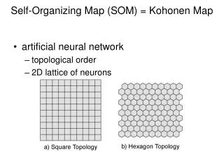
Self-Organizing Map (SOM) • 2D Grid of Output Nodes • Each output corresponds to an ideal input value • Inputs can be anything with a distance function • Activating an Output • Present input to the network • Output with the closest ideal input is the “winner”
Applying the SOM • Each input is a vector of sensor values • Sonar • Left/Right Bump Sensors • Left/Right Motor Speeds • Distance function is sum-of-squared-differences
SOM Unsupervised Learning • Present an input to the network • Find the winning output node • Update ideal input for winner and neighbors • weightij = weightij + (α * (inputij – weightij)) • Neighborhood function
Experiments • Implemented in Java (LeJOS 0.85) • Each experiment • 240 seconds (800 Q-Learning iterations) • 36 States • Three actions • Both motors forward • Left motor backward, right motor stopped • Left motor stopped, right motor backward
Rewards • Either bump sensor pressed: 0.0 • Base reward: • 1.0 if both motors are going forward • 0.5 otherwise • Multiplier: • Sonar value greater than 20 cm: 1 • Otherwise, (sonar value) / 20
Parameters • Discount (γ): 0.5 • Learning rate (α): • 1/(1 + (t/100)), t is the current iteration (time step) • Used for both SOM and Q-Learning [Smith 2002] • Exploration/Exploitation • Epsilon = α/4 • Probability of random action • Selected using weighted distribution
Experimental Controls • Q-Learning without SOM • Qa States • Current action (1-3) • Current bumper states • Quantized sonar values (0-19 cm; 20-39; 40+) • Qb States • Current bumper states • Quantized sonar values (9) (0-11 cm…; 84-95; 96+)
SOM Formulations • 36 Output Nodes • Category “a”: • Length-5 input vectors • Motor speeds, bumper values, sonar value • Category “b”: • Length-3 input vectors • Bumper values, sonar value • All sensor values normalized to [0-100]
SOM Formulations • QSOM • Based on [Smith 2002] • Gaussian Neighborhood • Neighborhood size is one-half SOM width • QT • Based on [Touzet 1997] • Learning rate is fixed at 0.9 • Neighborhood is immediate Manhattan neighbors • Neighbor learning rate is 0.4
Qualitative Results • QSOMa • Motor speeds ranged from 2% to 50% • Sonar values stuck between 90% and 94% • QSOMb • Sonar values range from 40% to 95% • Best two runs arguably the best of the bunch • Very smooth SOM values in both cases
Qualitative Results • QTa • Sonar values ranged from 10% to 100% • Still a weak performer on average • Best performer similar to QTb • QTb • Developed bump-sensor oriented behavior • Made little use of sonar • Highly uneven SOM values in both cases
First Movie • QSOMb • Strong performer (Reward: 661.89) • Minimum sonar value: 43.35% (110 cm)
Second Movie • Also QSOMb • Typical bad performer (Reward: 451.6) • Learns to avoid by always driving backwards • Baseline “not-forward” reward: 400.0 • Minimum sonar value: 57.51% (146 cm) • Hindered by small filming area
Discussion • Use of SOM on NXT can be effective • More research needed to address shortcomings • Heterogeneity of sensors is a problem • Need to try NXT experiments with multiple sonars • Previous work involved homogeneous sensors • Approachable by undergraduate students • Technique taught in junior/senior AI course