Download
1 / 41
410 likes | 509 Views
Modeling and Associated Visualization Needs. A Trilogy in Four Parts. The Acts: Not in Chronological Order. Overview of the G2P cyberinfrastructure Systems biology models (bottom up) Viz needs: Multivariate Dynamics, Inner Space, & Sensitivity Analysis Ecophysiological models (top down)

E N D
Modeling and Associated Visualization Needs A Trilogy in Four Parts
The Acts: Not in Chronological Order • Overview of the G2P cyberinfrastructure • Systems biology models (bottom up) • Viz needs: Multivariate Dynamics, Inner Space, & Sensitivity Analysis • Ecophysiological models (top down) • Viz needs: The same, plus Outer Space • Statistical models (non-mechanistic) • Viz needs: Help & fast!!
Solving the G2P problem means developing a methodology… …that lets one start with some species & trait that one knows very little about and end with the ability to quantitatively predict trait scores for target genotype/environment combinations. Build quantitative models Acquire data Ignorance Prediction Tools Elicit hypotheses Testing To work, such a methodology must be cyber-enabled
Seq data DI DI DI DI DI Expression data Data Visualization Visualization Metabolic data Whole plant data Environment data Super-user Developer Modeling and Statistical Inference Output Computational User inferred User inferred Hypothesis Experiment
Temperature Controlled by the amounts of upstream regulatory gene products Amount of gene product at time t Some fraction of M degrades per unit time Modeling a single gene
Linking multiple genes… Transcription Transcription Factor “A” Gene Codons DNA RNAP Promoter Region Translation Prot. Syn. “B” Gene Codons DNA RNAP PromoterRegion
Temperature modulates all rates Transcription Factors modulate reading Other Gene Products affect degradation Gene Product A Gene Product B A “Bathtub” Model
What is a “product”? • RNA’s: messenger (mRNA) & otherwise • Some models do not distinguish mRNA & protein (e.g., when time scales are long) • Some models individually represent mRNA, cytosolic protein, and nuclear protein • Some models will separate products by tissue/organ (e.g., leaves, phloem, meristem) • Many models include metabolites & protein complexes • Basic equation is still the same (influx-eflux)
Linear Constant Frac. Hill Function Michaelis-Menton Activation Input Mass Action Etc.
Folded protein packaged to go Chaperone (folds/QC) Bad protein (unreleased) Endoplasmic reticulum (Abstracted from Ellgaard et al. 1999) One form of temperature effect
Linear Constant Frac. Hill Function Michaelis-Menton Activation Input Mass Action Etc. Temperature effects
Michaelis-Menton Mass action Influx - Efflux Translation Hill function mRNA Environmental effect (light) Net transport into nucleus ? Locke et al., 2005 - 9 of 13 equations A close up – the diurnal clock Locke et al., 2005 Barak et al., 2000
Sensitivity Analysis & Sloppy Systems Each letter is a power of two in sensitivity
All parameter combinations inside this ellipse yield essentially identical goodness-of-fit values Optimum goodness-of-fit “Sloppy” direction “Stiff” direction Stiff & Sloppy Directions Parameter 2 Sloppy/Stiff ca. 1000 Parameter 1 The “ellipses” may be “hyper-pancakes” with 15 to 30 sloppy directions. How can these be meaningfully visualized??
GIGANTEA ? Sloppy directions in a clock model 71 parameters reduced to 46 parameters
Ecophysiological Models… • …come in three flavors • Environmental physics models (1945 to present) • Crop simulation models (1965 to present) • Geochemical cycling models • Blend the characteristics of both of the above • Are more recent • …are now poised to contribute to the G2P problem via a top-down approach
What is the focus of models in Environmental Physics? • Mimics conditions inside a uniform plant canopy; • The typical setting is an agricultural field; • Includes plant-related, edaphic (soil), and meteorological inputs; • Based on physical principles; • Conservation of matter and energy; convection, conduction, convection; • Some plant processes – gas exchange, photosynthesis, respiration • Plant structure consists of leaves, stems, roots; • Time horizon typically a few days with time steps on the order of minutes. • Ergo plants often do not grow
Environmental Physics Models: 1945-75 • 1D or Bulk approach; • Big Leaf / Big Root submodels; • Bucket soil submodels; • Resistance analogs used for the atmospheric environment; • Limited prediction of soil or canopy scalar variables; • Many empirical relationships; • Nebulous controlling variables (e.g., canopy resistance to vapor flux); • Poor plant/environment feedback. Atmosphere Big Leaf Bucket of Soil Big Root
Environmental Physics Models: 1975-90 • Multi-layer atmosphere, soil, and canopy; • “Scaled leaf” approach within canopy layers; • Relationships between photo-synthesis, transpiration, and biophysics (e.g., stomatal action); • Use finite difference methods to compute soil heat, water, and gas flows; • Incorporate root density functions and soil physical properties. TAIR , VPD, CO2 , wind speed profiles Atmosphere Layers Canopy Layers Sunlit TCANOPY , VPD, CO2 , canopy profiles Shade Soil Layers TSOIL , profiles Rooting Profile
What is a Crop Growth Model? • Mimics one “average plant” at a field or smaller scale; • The plant environment is an agricultural production setting; • Includes cultural- and production-related I/O variables; • Includes varietal, edaphic, and meteorological inputs; • Based on physiological processes; • Photosynthesis, respiration, transpiration, nutrient uptake, carbon partitioning, growth, and phenological development; • Plant structure consists of leaves, stems, roots, & grain; • Annual time horizon with daily or hourly time steps.
What is the current status of Crop Growth Models? • Skillful models can account for ca. 70% of yield variance; • Ongoing work focuses on refinement and applications; • Problems being researched include methods for estimating cultivar and soil characteristics on an operational scale; • Model structures and approaches have matured; • Recent physical theory may not be emphasized; • Physical theory does not seem to improve predictions. • Interestingly, incorporating crop growth model components into physical models does not guarantee improved predictability either, even though physical scientists recognize knowledge of the plant as limiting.
Special case Geochemical cycling models • Used to model “ecosystem services” and/or “land surface processes” inside general circulation models • Blend of both kinds of models; • Includes plant-related, edaphic, and meteorological inputs; • Based on physical principles • Conservation of matter and energy; convection, conduction, convection; • Some plant processes – gas exchange, photosynthesis, respiration • Plant structure consists of leaves, stems, roots; • Time horizon of years with time steps on the order of minutes (depends on spatial scale).
Main points -- • Neither current crop growth models nor environmental physics models adequately depict plant process control mechanisms; • This accounts for the failure of models to mimic the plasticity of real plants across different environments; • The information needed to remedy this situation is emerging from the genomic sciences; • Incorporating this information requires a reorganization of crop models
New Crop Growth Model Concept Energy Water N Sensors [KE60] Control Submodel Physical Submodel [CPAI]
Viz needs for ecophysiological models and G2P components • Largely the same as for systems biology models – multivariate dynamics in spatially discrete plant parts • Note that our “G2P solution” specifies predicting trait scores in non-constant environments. • That most directly refers to the outdoors • Therefore geographic variation must also be considered
A hazy shade of winter… • One frame of a movie comparing the standard deviation of flowering time for the Columbia strain of A. thaliana germinating on each day. • Projected by the gene-based model of Wilczek et al, 2009. • The standard deviation is over five years (left, 2004-2009, real data; right, 2094-2099, A1B climate scenario.)
Statistical genetic methods I • Can be used to • Predict phenotypes based on genotypes • Locate regions of the genome likely to contain genes controlling particular phenotypes • Can be used when • Knowledge of gene mechanisms is lacking • Big Caveat • The mathematical form of the G2P relationship is just assumed to be linear • … and the data & models elaborated until the job gets done to adequate accuracy
Statistical genetic methods II • Why does it work? • Because there are sufficient regimes of near linearity buried in mechanistic network eq’ns that general linear statistical models have levels of predictive skill useful for some purposes (e.g. crop breeding) • Rest assured that there are limits to what should be expected of these models • How does it work?
What are genetic markers? Position within gene Aligned DNA sequences of 25 different genetic lines Single nucleotide polymorphism (SNP) (Data from the Purugganan Lab)
Different sibling lines will have different marker combinations The DNA sequence for line 1 has the same sequence as parent “B” at the location of marker “g17286”… …but in line 8 the DNA matches parent “A” at that location
Genome Wide Association Finding quantitative trait loci (QTL) Find markers i, j, and k such that is a good fit Many different linear models etc….
What a QTL analysis output looks like. This is a “1d-scan” – i.e. Xm,j (Buckler et al, Science, 2009)
Two Stat Inf Viz Problems • Higher order scans e.g. • Remember SNP numbers can be in the 150K to 3M range. • eQTL viz problems • Can be 30K phenotypes… • …and higher order scans
eQTL Analysis – Looking for Regulators Transcription Factor “A” Gene Codons DNA RNAP Promoter Region Prot. Syn. “B” Gene Codons DNA RNAP PromoterRegion Let “Pheno” be the amount of mRNA (expression) produced by gene “B”. This could be different in lines that varied either in the promoter of “B” or in lines that had differences in the coding region of gene “A”. These are called “cis” and “trans” effects, respectively.
Massive eQTL Variation75% of all genes have at least 1 eQTL Cis Diagonal Chromosome I II III IV V QTL Effect Bay + Bay - Position of eQTL for each of 15,771 genes Arranged by Physical Order (D. Kliebenstein) Trans Hotspot
eQTL Viz Problems… How to plot interaction effects? That is Xm,jXm,k and a gazillion phenotypes
Questions? Virtual soybean simulations from Han et al. 2007