Transportation and Assignment Model s

1. Transportation and Assignment Models

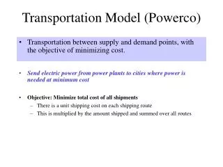
2. Transportation Models • Transportation probleminvolve determining how to optimally (minimum shipping cost) transport goods from the sources to destinations. • Usually we are given the capacity of goods at each source and the requirements at each destination • Typically the objective is to minimize total transportation and production costs

3. Consider the case given below. There are sources (Albuquerque, Boston and Cleveland) and there are destinations (Des Moines Evansville and Fort Lauderdale) with costs, and constraints for capacity and demand.

5. Basic feasible solution can be obtained by three methods, they are • North - west corner method, • Least - cost cell method, • Vogel's Approximation Method, generally known as VAM.

6. After getting the basic feasible solution, do optimality test to check whether the solution is optimal or not. There are two methods of doing optimality test, they are • Stepping Stone Method, • Modified Distribution Method, generally known as MODI method.

7. Properties of a Basic feasible Solution • It must satisfy availability constraints and requirement constraints. • It should satisfy non negativity constraint. • Total number of allocations must be equal to (m + n – 1), where 'm' is the number of rows and 'n' is the number of columns.

8. Initial Solution with NORTH-WEST corner method

9. Step1Start from the left hand side top corner or cell and make allocations depending on the availability and requirement constraint.

10. Step 2By satisfying availability and requirement constraints fill the other cells. Z=1005 + 2008+1004+1007+2005=500+1600+400+700+1000=4200 $

11. Initial Solution with LEAST COST method • Identify the lowest cost cell in the given matrix. In this particular example it is 3. Make allocations to this cell. After filling search for lowest cost cell. Proceed this way until all allocations are made. Z=3009+2004+1003+1003=2700+800+300+300=4100 $

12. Initial Solution with Vogel’s Approximation Method (VAM) • Step 1:For each row and column find the difference between the two lowest unit shipping costs.

13. Step 2 Assign as many units as possible to the lowest-cost square in the row and column selected.

14. Step 3Eliminate the column or row that has been satisfied.

16. Z= 1005+2004+1003+2009+1005=500+800+300+1800+500=3900 $

17. STEPPING STONE METHOD of optimality test Once, we get the basic feasible solution for a transportation problem, the next duty is to test whether the solution we got is an optimalsolution or not? • Steps to test unused squares; • Select an unused square, • Allocate +①unit to unused square and locate -① and +① alternatively to corners of the selected closed path, • Calculate the improvement index , • If improvement index is negative allocate as much as you can to that unused square, • Repeat the allocation till the improvement index is ≥0 for all unused squares.

18. Application of the Method:

22. Since there is a decrease in the cost, we will allocate as much as we can to Fort Lauderdale – Albuquerque. The amount is the minimum of the numbers that we are assigning -① in the cycle. Z=1005 + 1008+2004+1009+2005=500+800+800+900+1000=4000 $

23. An improvement can be done by allocating to EC, since the minimum number in the square is 100; we allocate 100 to EC square.

24. Z=1005 + 2009+2004+1003+1005=500+1800+800+300+500=3900 $ We will check the Improvement index in each cell again. In the table, no more negative improvement index, so the solution is optimal.

25. Example A company has three factories X, Y, and Z and three warehouses A, B, and C. It is required to schedule factory production and shipments from factories to warehouses in such a manner so as to minimize total cost of shipment and production. Unit variable manufacturing cost (UVMC) and factory capacities and warehouse requirements are given below: a) Load the table with North-west method. b) Load the table with least cost method. c) Load the table with Vogel’s approximation method, (VAM). d) Solve the question by stepping stone algorithm.

26. Example The demand and capacity are given. a) Load the table with North-west method. b) Load the table with least cost method. c) Load the table with Vogel’s approximation method, (VAM). d) Solve the question by stepping stone algorithm.

27. Assignment Model • Allocating one person to one job and minimizing the time or cost of problem is solved by ASSIGNMENT MODEL. • The assignment problem refers to the class of LP problems that involve determining the most efficient assignment of resources to tasks • The objective is most often to minimize total costs or total time to perform the tasks at hand

28. There are n!=4!=432 1=24 number of solutions. If there is 5 assignment there will be 5!=120 different combinations.Therefore , instead of writing all the combinations, an algorithm (Hungarian Method) will be used to find the solution.

29. Hungarian Method • The Hungarian method is an efficient method of finding the optimal solution to an assignment problem without having to make direct comparisons of every option • It operates on the principle of matrix reduction • By subtracting and adding appropriate numbers in the cost table or matrix, we can reduce the problem to a matrix of opportunity costs • Opportunity costs show the relative penalty associated with assigning any person to a project as opposed to making the best assignment • We want to make assignment so that the opportunity cost for each assignment is zero

30. There are five steps to find the optimum result.

33. Step4. If the lines drawn are less than the number of rows or columns, then we cannot make assignment. Hence the following procedure is to be followed: - The cells covered by the lines are known as Covered cells. - The cells, which are notcovered by lines, are known as uncovered cells. - The cells at the intersection of horizontal line and vertical lines are known as Crossed cells. (a) Identify the smallest element in the uncovered cells. (i)Subtract this element from the elements of all other uncovered cells. (ii) Add this element to the elements of the crossed cells. (iii) Do not alter the elements of covered cells. (b) Once again cover all the zeros by minimum number of horizontal and vertical lines. (c) Once the lines drawn are equal to the number of rows or columns, assignment can be made.

36. Example There are 3 jobs A, B, and C and three machines X, Y, and Z. All the jobs can be processed on all machines. The time required for processing job on a machine is given below in the form of matrix. Make allocation to minimize the total processing time.