Download
1 / 14
140 likes | 297 Views
The transportation model. A special case of the linear programming mode l. The transportation problem. …i nvolves finding the lowest-cost plan for distributing stocks of supplies from multiple origins to multiple destinations that demand them. The optimal shipping plan.

E N D
The transportation model A special case of the linear programming model
The transportation problem • …involves finding the lowest-cost plan for distributing stocks of supplies from multiple origins to multiple destinations that demand them.
The optimal shipping plan • The transportation model is used to determine how to allocate the supplies available at the origins to the customers, in such a way that total shipping cost is minimized. • The optimal set of shipments is called the optimal shipping plan. • There can be more optimal shipping plans. • The plan will change if any of the parameters changes significantly.
A possible transportation problem situation D D S S D S D
Defining the classic transportation problem The goods have more shipping points (suppliers) and more destinations (buyers). Prices are fixed. The sum of the quantities supplied and the sum of quantities demanded are equal. There are no surpluses nor shortages. ai and bj are both positive (there are no reverse flow of goods) the dependent variables are the transported quantities form origin i to destination j: xij≥ 0 All of the supplies should be sold and all of the demand should be satisfied. Tha aim is to minimize the total transportation cost: Homogeneous goods. Shipping costs per unit are constant. Only one route and mode ofg transportation exists between each origin and each destination.
Typical areas of transportation problems • Suppliers of components and assembly plants. • Factories and shops. • Suppliers of raw materials and factories. • Food processing factories and food retailers.
Informations needed to built a model • A list of the shipping points with their capacities (supply quantities). • A list of the destinations with their demand. • Transportation costs per unit from each origin to each destination • Question: what if prices of the good are differ form supplier to supplier?
Surplus If the total supply is greater than the total demand, than we have to add a ‘phantom’ destination to the model the demand of which is equal to the surplus. The transportation cost to this phantom destination is 0 from every supplier. De quantities shipped to this virtual customer will be those that will not be bought by anybody.
Shortages The formal solution is the same as it was in the case of a surplus (with 0 transportation costs): But: mathematics are less adequate in the case of shortages than in the case of surplusses, because of the consequences.
Solving transportation problems • Never try without a computer • There can be many equivalent solutions (with the same total cost).