Download
1 / 30
320 likes | 444 Views
time varying. Two asymptotic techniques are. Large dim. of x is another. Averaging takes care of ; Singular perturbation takes care of . Asymptotic Techniques. Introduction. Real world complex for a direct analysis. Solution simplification.

E N D
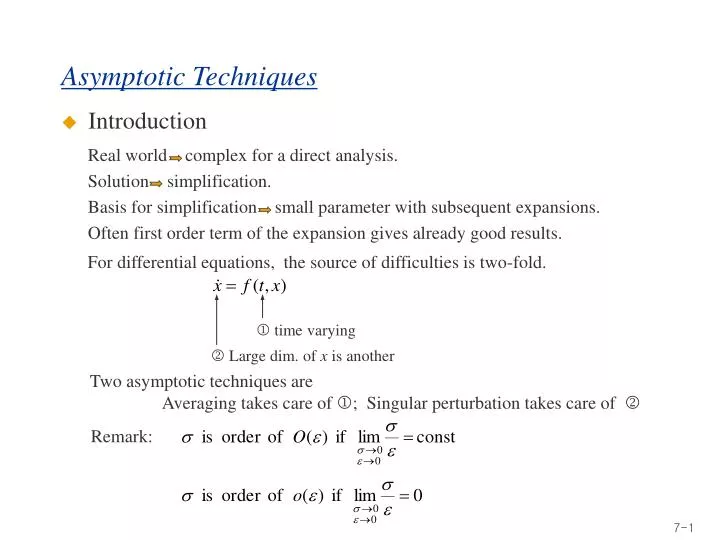
time varying Two asymptotic techniques are Large dim. of x is another Averaging takes care of ; Singular perturbation takes care of Asymptotic Techniques • Introduction Real world complex for a direct analysis. Solution simplification. Basis for simplification small parameter with subsequent expansions. Often first order term of the expansion gives already good results. For differential equations, the source of difficulties is two-fold. Remark:
Averaging • Averaging • Motivation Ex: Consider the system
Averaging (Continued) source of difficulties Averaging will get rid of this !
Averaging (Example) Then the averaged equation is Asymptotically stable Ex: (1)
Example (Continued) To get rid of it, we use the idea of generating equation Solve it. Introduce the substitution.
Example (Continued) Then, from (1) or Thus Thus again, what we obtained is So if we will be able to analyze such systems in a simple basis, we will solve the system
Example (Continued) The average equations are In the original time or Equation point
Stability analysis Stability analysis (i) (ii)
Theory • Theory slow variable fast variable
Theorem 1 Theorem 1
Theorem 2 Theorem 2
Theorem 3 Theorem 3 Ex: Van der Pol eq.
Example Ex:
Singular Perturbations • Singular Perturbations • Idea
Example Ex:
Example Ex:
Theory • Theory Conditions
Theorem Theorem:
Example Ex:
Linear Systems • Linear Systems
NonLinear Systems • Nonlinear Systems Theorem Proof : See Nonlinear Systems Analysis.
Example Ex:
find state feedback dynamic output feedback Nonlinear Control • Indeed, Why do we use nonlinear control : • Modify the number and the location of the steady states. • Ensure the desired stability properties • Ensure the appropriate transients • Reduce the sensitivity to plant parameters Remark: Consider the following problem :
Nonlinear Control Vs. Linear Control • Why not always use a linear controller ? • It just may not work. Ex: Choose Then We see that the system can’t be made asymptotically stable at On the other hand, a nonlinear feedback does exist : Then Asymptotically stable if
+ _ Example • Even if a linear feedback exists, nonlinear one may be better. Ex: + _
If If Let us use a nonlinear controller : To design it, consider again Example (Continued)
Switch from to appropriately and obtain a variable structure system. Example (Continued) sliding line Created a new trajectory: the system is insensitive to disturbance in the sliding regime Variable structure control