Download
1 / 37
400 likes | 585 Views
Asymptotic Analysis. Asymptotic Analysis Instructor: George Bebis (Chapter 3, Appendix A). Analysis of Algorithms. An algorithm is a finite set of precise instructions for performing a computation or for solving a problem. What is the goal of analysis of algorithms?

E N D
Asymptotic Analysis Asymptotic Analysis Instructor: George Bebis (Chapter 3, Appendix A)
Analysis of Algorithms • An algorithm is a finite set of precise instructions for performing a computation or for solving a problem. • What is the goal of analysis of algorithms? • To compare algorithms mainly in terms of running time but also in terms of other factors (e.g., memory requirements,programmer's effort etc.) • What do we mean by running time analysis? • Determine how running time increases as the size of the problem increases.
Input Size • Input size (number of elements in the input) • size of an array • polynomial degree • # of elements in a matrix • # of bits in the binary representation of the input • vertices and edges in a graph
Types of Analysis • Worst case • Provides an upper bound on running time • An absolute guarantee that the algorithm would not run longer, no matter what the inputs are • Best case • Provides a lower bound on running time • Input is the one for which the algorithm runs the fastest • Average case • Provides a prediction about the running time • Assumes that the input is random
How do we compare algorithms? • We need to define a number of objective measures. (1) Compare execution times? Not good: times are specific to a particular computer !! (2) Count the number of statements executed? Not good: number of statements vary with the programming language as well as the style of the individual programmer.
Ideal Solution • Set of primitive operations: • Arithmetic. Logical, Comparisons, Function calls • Simplifying assumption: all ops cost 1 unit • Eliminates dependence on the speed of our computer, otherwise impossible to verify and to compare • Express running time as a function of the input size n (i.e., f(n)). • Compare different functions corresponding to running times. • Such an analysis is independent of machine time, programming style, etc.
Example • Associate a "cost" with each statement. • Find the "total cost“by finding the total number of times each statement is executed. Algorithm 1 Algorithm 2 Cost Cost arr[0] = 0; c1 for(i=0; i<N; i++) c2 arr[1] = 0; c1 arr[i] = 0; c1 arr[2] = 0; c1 ... ... arr[N-1] = 0; c1 ----------- ------------- c1+c1+...+c1 = c1 x N(N+1) x c2 + N x c1 = (c2 + c1) x N + c2
Another Example • Algorithm 3 Cost sum = 0; c1 for(i=0; i<N; i++) c2 for(j=0; j<N; j++) c2 sum += arr[i][j]; c3 ------------ c1 + c2x (N+1) + c2x N x (N+1) + c3x N2
Asymptotic Analysis • To compare two algorithms with running times f(n) and g(n), we need a rough measure that characterizes how fast each function grows. • Hint: use rate of growth • Compare functions in the limit, that is, asymptotically! (i.e., for large values of n)
Rate of Growth • Consider the example of buying elephants and goldfish: Cost: cost_of_elephants + cost_of_goldfish Cost ~ cost_of_elephants (approximation) • The low order terms in a function are relatively insignificant for largen n4 + 100n2 + 10n + 50 ~ n4 i.e., we say thatn4 + 100n2 + 10n + 50 and n4 have the same rate of growth
Asymptotic Notation • O notation: asymptotic “less than”: • f(n)=O(g(n)) implies: f(n) “≤” g(n) • notation: asymptotic “greater than”: • f(n)= (g(n)) implies: f(n) “≥” g(n) • notation: asymptotic “equality”: • f(n)= (g(n)) implies: f(n) “=” g(n)
Big-O Notation • We say fA(n)=30n+8is order n, or O (n) It is, at most, roughly proportional to n. • fB(n)=n2+1 is order n2, or O(n2). It is, at most, roughly proportional to n2. • In general, any O(n2) function is faster- growing than any O(n) function.
Visualizing Orders of Growth • On a graph, asyou go to theright, a fastergrowingfunctioneventuallybecomeslarger... fA(n)=30n+8 Value of function fB(n)=n2+1 Increasing n
More Examples … • n4 + 100n2 + 10n + 50 is O(n4) • 10n3 + 2n2 is O(n3) • n3 - n2 is O(n3) • constants • 10 is O(1) • 1273 is O(1)
Back to Our Example Algorithm 1 Algorithm 2 Cost Cost arr[0] = 0; c1 for(i=0; i<N; i++) c2 arr[1] = 0; c1 arr[i] = 0; c1 arr[2] = 0; c1 ... arr[N-1] = 0; c1 ----------- ------------- c1+c1+...+c1 = c1 x N (N+1) x c2 + N x c1 = (c2 + c1) x N + c2 • Both algorithms are of the same order: O(N)
Example (cont’d) Algorithm 3 Cost sum = 0; c1 for(i=0; i<N; i++) c2 for(j=0; j<N; j++) c2 sum += arr[i][j]; c3 ------------ c1 + c2x (N+1) + c2x N x (N+1) + c3x N2= O(N2)
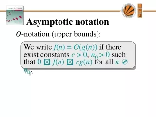
Asymptotic notations • O-notation
Big-O Visualization O(g(n)) is the set of functions with smaller or same order of growth as g(n)
Examples • 2n2 = O(n3): • n2 = O(n2): • 1000n2+1000n = O(n2): • n = O(n2): 2n2≤ cn3 2 ≤ cn c = 1 and n0= 2 n2≤ cn2 c ≥ 1 c = 1 and n0= 1 1000n2+1000n ≤ 1000n2+ n2 =1001n2 c=1001 and n0 = 1000 n ≤ cn2 cn ≥ 1 c = 1 and n0= 1
More Examples • Show that 30n+8 is O(n). • Show c,n0: 30n+8 cn, n>n0. • Let c=31, n0=8. Assume n>n0=8. Thencn = 31n = 30n + n > 30n+8, so 30n+8 < cn.
cn =31n n>n0=8 Big-O example, graphically • Note 30n+8 isn’tless than nanywhere (n>0). • It isn’t evenless than 31neverywhere. • But it is less than31neverywhere tothe right of n=8. 30n+8 30n+8O(n) Value of function n Increasing n
No Uniqueness • There is no unique set of values for n0 and c in proving the asymptotic bounds • Prove that 100n + 5 = O(n2) • 100n + 5 ≤ 100n + n = 101n ≤ 101n2 for all n ≥ 5 n0 = 5 and c = 101is a solution • 100n + 5 ≤ 100n + 5n = 105n ≤ 105n2for all n ≥ 1 n0 = 1 and c = 105is also a solution Must findSOMEconstants c and n0 that satisfy the asymptotic notation relation
Asymptotic notations (cont.) • - notation (g(n)) is the set of functions with larger or same order of growth as g(n)
Examples • 5n2 = (n) • 100n + 5 ≠(n2) • n = (2n), n3 = (n2), n = (logn) cn 5n2 c = 1 and n0 = 1 • c, n0such that: 0 cn 5n2 c, n0 such that: 0 cn2 100n + 5 100n + 5 100n + 5n ( n 1) = 105n cn2 105n n(cn – 105) 0 n 105/c Since n is positive cn – 105 0 contradiction: n cannot be smaller than a constant
Asymptotic notations (cont.) • -notation • (g(n)) is the set of functions with the same order of growth as g(n)
Examples • n2/2 –n/2 = (n2) • ½ n2 - ½ n ≤ ½ n2n ≥ 0 c2= ½ • ½ n2 - ½ n ≥ ½ n2 - ½ n * ½ n ( n ≥ 2 ) = ¼ n2 c1= ¼ • n ≠ (n2): c1 n2≤ n ≤ c2 n2 only holds for: n ≤ 1/c1
Examples • 6n3 ≠ (n2): c1 n2≤ 6n3 ≤ c2 n2 only holds for: n ≤ c2 /6 • n ≠ (logn): c1logn≤ n ≤ c2 logn c2 ≥ n/logn, n≥ n0 – impossible
Relations Between Different Sets • Subset relations between order-of-growth sets. RR ( f ) O( f ) • f ( f )
Logarithms and properties • In algorithm analysis we often use the notation “log n” without specifying the base Binary logarithm Natural logarithm
More Examples • For each of the following pairs of functions, either f(n) is O(g(n)), f(n) is Ω(g(n)), or f(n) = Θ(g(n)). Determine which relationship is correct. • f(n) = log n2; g(n) = log n + 5 • f(n) = n; g(n) = log n2 • f(n) = log log n; g(n) = log n • f(n) = n; g(n) = log2 n • f(n) = n log n + n; g(n) = log n • f(n) = 10; g(n) = log 10 • f(n) = 2n; g(n) = 10n2 • f(n) = 2n; g(n) = 3n f(n) = (g(n)) f(n) = (g(n)) f(n) = O(g(n)) f(n) = (g(n)) f(n) = (g(n)) f(n) = (g(n)) f(n) = (g(n)) f(n) = O(g(n))
Properties • Theorem: f(n) = (g(n)) f = O(g(n)) and f = (g(n)) • Transitivity: • f(n) = (g(n))andg(n) = (h(n)) f(n) = (h(n)) • Same for O and • Reflexivity: • f(n) = (f(n)) • Same for O and • Symmetry: • f(n) = (g(n)) if and only if g(n) = (f(n)) • Transpose symmetry: • f(n) = O(g(n)) if and only if g(n) = (f(n))
Asymptotic Notations in Equations • On the right-hand side • (n2) stands for some anonymous function in (n2) 2n2 + 3n + 1 = 2n2 + (n) means: There exists a function f(n) (n) such that 2n2 + 3n + 1 = 2n2 + f(n) • On the left-hand side 2n2 + (n) = (n2) No matter how the anonymous function is chosen on the left-hand side, there is a way to choose the anonymous function on the right-hand side to make the equation valid.
Common Summations • Arithmetic series: • Geometric series: • Special case: |x| < 1: • Harmonic series: • Other important formulas:
Mathematical Induction • A powerful, rigorous technique for proving that a statement S(n) is true for every natural number n, no matter how large. • Proof: • Basis step: prove that the statement is true for n = 1 • Inductive step: assume that S(n) is true and prove that S(n+1) is true for all n ≥ 1 • Find case n “within” case n+1
Example • Prove that: 2n + 1 ≤ 2n for all n ≥ 3 • Basis step: • n = 3: 2 3 + 1 ≤ 23 7 ≤ 8 TRUE • Inductive step: • Assume inequality is true for n, and prove it for (n+1): 2n + 1 ≤ 2nmust prove: 2(n + 1) + 1 ≤ 2n+1 2(n + 1) + 1 = (2n + 1 ) + 2 ≤ 2n + 2 ≤ 2n + 2n = 2n+1, since 2 ≤ 2nfor n ≥ 1