Download
1 / 103
1.13k likes | 1.38k Views
Hydrologic trend analysis. Dennis P. Lettenmaier Department of Civil and Environmental Engineering University of Washington GKSS School on Statistical Analysis in Climate Research Lecce, Italy October 15, 2009. Outline of this talk. Water cycle observations

E N D
Hydrologic trend analysis Dennis P. Lettenmaier Department of Civil and Environmental Engineering University of Washington GKSS School on Statistical Analysis in Climate Research Lecce, Italy October 15, 2009
Outline of this talk Water cycle observations Long-term trend analysis of hydrologic variables Nonparametric approach (seasonal Man n Kendall) Examples Some pitfalls in trend analysis Analysis and trends in hydrologic extremes
Land surface water balance Atmospheric water balance Land surface and atmospheric water and energy balances both contain evapotranspiration (with a multiplier) 1. Water cycle observations
In situ methods use gauges (essentially points) Issues with representativeness, changes of instrumentation in time, biases (see Phil Jones lecture) Wind catch deficiency is critical problem for solid precipitation, of somewhat lesser (but not necessarily negligible) magnitude Small scale spatial variability (tends to average out with time) Surface radars Provides near spatially continuous coverage Terrain blockage issues, also tilt angle, other issues Complications in producing climate quality records Remote sensing Indirect (aside from TRMM radar) Sampling issues aside from geostationary Solid precipitation issues Precipitation measurement (dominant hydrological forcing)
Stream discharge (streamflow) measurement Stage (water height), not discharge is measured. Discharge is derived via a (usually power law) rating curve derived from discrete stage and discharge measurements, applied to time-continuous stage measurements Visuals courtesy USGS
Snow Water Equivalent (SWE) measurement – manual snow courses Visuals courtesy NRCS
SWE measurement – automated snow pillows Enhanced SnoTEL installation Typical SnoTEL installation Visuals courtesy NRCS
Soil moisture few climate quality observations with consistent observation methods In situ methods are complicated by short scale (as small as 1 m) spatial variability Evapotranspiration Most common long-term measurement is pan evaporation, which can be considered a rough index to potential (not actual) evapotranspiration Flux towers (AmeriFlux, EuroFlux, FluxNet) provide estimates of latent heat flux (essentially actual evapotranspiration) via either eddy correlation or Bowen ratio methods. However, record lengths are short from a climatological perspective, and generally not of trend quality Groundwater Relatively few well observations of long length that are not affected by management (withdrawals) Satellite (GRACE) data provide an alternative over large areas, but record is short (less than a decade), and measurement is effectively all changes in moisture content (atmospheric, soil moisture, lakes, etc) Lakes and wetlands Very few records suitable for trend analysis Some work on high latitude lakes (surface area) from remote sensing Glaciers Relatively small number of glaciers have detailed mass balance records, but many changes are not subtle Changes in area are generally easier to detect than storage (and are amenable to visible satellite imagery with record lengths exceeding 30 years Satellite altimetry (e.g. ICESAT) provides basis for storage estimates, but record lengths are short Other hydrological variables
Precipitation: usually measured as accumulations over time, statistics are characterized by intermittency and high Cv and skewness for accumulation intervals < multiple days. Correlation lengths increase with accumulation intervals, generally greater for winter (synoptic scales events) than summer (convective); skewness and Cv decrease with accumulation intervals (and intemittency vanishes) Streamflow: Most variable of land surface fluxes; can be intermittent for short accumulation intervals in arid areas and in some cases small drainage areas. Controls include precipitation and evaporative demand, but also land surface characteristics and drainage areas. It is an areal integrator. Spatial correlation lengths usually longer than for precipitation. Evapotranspiration: Least variable of three major land surface hydrologic fluxes. Near-direct measurement difficult, and mostly applicable to points, large area estimates from remote sensing (essentially indirect/model), or by difference Soil moisture: Few long-term observations available, most viable approach (not without shortcomings) is model reconstruction Groundwater: Few long-term observations available that are not dominated by management effects; large area estimates (which include other storage terms) now possible via satellite microgravity (GRACE) Snow water equivalent: Point measurements from snow courses (now increasingly replaced with automated snow pillows) Hydrologic data characteristics
Testing for Trends Ho: Distribution (F) of R.V. Xt is same for all t H1: F changes systematically with time We may also want to describe the amount or rate of change, in property (e.g. central tendency) of the distribution
Parametric vs Nonparametric statistics Parametric: Assume the distribution of Xt (often Gaussian) Nonparametric: Form of distribution not assumed (but often are some assumptions, e.g. common distribution aside from change in central tendency) Nonparametrictests are usually more robust to violation of assumptions that must be made for parametric tests, however when parametric tests are appropriate, the range of quantitative inferences that can be made is usually greater
Monotonic Trend: Continuing (and not reversing) with time Parametric test example: linear regression (with time) Nonparametric test examples: Kendall’s tau; spearman’s rho (essentially rank correlation with time)Step Trend: One-time change, of fixed amount Parametric test example: t-test Non-parametric test example: Mann Whitney
Kendall’s Tau (t) • Tau (t) measures the strength of the monotonic relationship between X and Y. Tau is a rank-based procedure and is therefore resistant to the effect of a small number of unusual values. • Because t depends only on the ranks of the data and not the values themselves, there are adjustments for missing or censored data (essentially treated as ties) – tests work with a “limited amount of” such data • In general, for linear associations, t < r. Strong linear correlations of r > 0.9 corresponds to t > 0.7. • For trend test, Y can be time
The test statistic S measures the monotonic dependence of X on t: • S = P - M • where : P = # of (+), the # of times the X’s increase with t, or the # of Xi < Xj for all ti < tj (“concordant pairs”). • M = # of (-), the # of times the X’s decrease with t, or the number of Xi > Xj for all ti <tj (“discordant pairs”). • i = 1, 2, … (n-1); and j = (i+1), …, n. • There are n(n-1)/2 possible comparisons to be made among the n data pairs. If all y values increased along the x values, S = n(n-1)/2. In this situation, t = +1, and vice versa. Therefore dividing S by n(n-1)/2 will give a -1 < t < +1. • Adjustment can be made for ties (missing or censored data)
t is defined as : • Critical value of S can be determined by enumerating the discrete distribution of S, when the data are randomly ranked with time • For n > about 10, there is a large sample approximation to the test statistic; for smaller values, tables of the exact distribution are available
Key assumptions for Kendall’s tau (or Mann-Kendall test) • Common distribution of Xt (most importantly homoscedastic) • Independence (no temporal correlation)
Large sample approximation • The large sample approximation Zs is given by: • And, Zs = 0, if S = 0, and where: • The null hypothesis is rejected at significance level a if Zs > Zcrit where Zcrit is the critical value of the standard normal distribution with probability of exceedance of a/2 (i.e., S is approximately normally distributed with mean 0).
Kendall slope estimator Med {(Xj-Xi)/(tj-ti)} for all j>I
Seasonality effects Usually result in violation of key assumption, as distributions of most hydrologic (and climatic) variables change with season One approach is to “homogenize” time series e.g. by seasonal transformation (can be left with issues as to seasonally varying correlation)
Seasonal Kendall Test (per Hirsch et al, 1982) where ti is number of ties in season i From Hirsch et al (1982)
Absent missing data (note that g is season index, p is number of seasons): Where rgh is Spearman’s rho (rank correlation) between seasons g and h
Mann Kendall analysis -- annual minimum flow from 1941-70 to 1971-99 Minimum flow Increase No change Decrease Visual courtesy Bob Hirsch, figure from McCabe & Wolock, GRL, 2002
Median flow Increase No change Decrease About 50% of the 400 sites show an increase in annual median flow from 1941-71 to 1971-99 Visual courtesy Bob Hirsch, figure from McCabe & Wolock, GRL, 2002
Maximum flow Increase No change Decrease About 10% of the 400 sites show an increase in annual maximum flow from 1941-71 to 1971-99 Visual courtesy Bob Hirsch, figure from McCabe & Wolock, GRL, 2002
USGS streamgage annual flood peak records used in study (all >=100 years) Visual courtesy Bob Hirsch
Number of statistically significant increasing and decreasing trends in U.S. streamflow (of 395 stations) by quantile (from Lins and Slack, 1999)
Annual hydroclimatic trends over the continental U.S., 1948-88 from Lettenmaier et al, 1994
Monthly streamflow trends over the continental U.S., 1948-88 from Lettenmaier et al, 1994
1925-2003 period selected to account for model initialization effects Positive trends dominate (~28% of model domain vs ~1% negative trends) Positive + Negative Drought trends in the continental U.S. – from Andreadis and Lettenmaier (GRL, 2006) Model Runoff Annual Trends
Trend direction and significance in streamflow data from HCN have general agreement with model-based trends HCN Streamflow Trends Subset of stations was used (period 1925-2003) Positive (Negative) trend at 109 (19) stations
Positive trends for ~45% of CONUS (1482 grid cells) Negative trends for ~3% of model domain (99 grid cells) Positive + Negative Soil Moisture Annual Trends
Spurious trends (e.g., changes in instruments; site-specific effects). Solution: understand the data and adjust as necessary; evaluate spatial consistency of trends (site specific effects should not have a spatial signature) Multiple comparison problem (“fishing expeditions”). Solution: test field significance; pre-specify the tests, time periods, etc to be tested. Strong conclusions from short record lengths (e.g. satellite data) 2.3 Pitfalls in trend analysis
References Fowler, H.J., and C.G. Kilsby, 2003. A regional frequency analysis of United Kingdom extreme rainfall from 1961 to 2000, International Journal of Climatology 23, 1313-1334. Hirsch, R.M., J.R. Slack, and R.A. Smith, 1982. Techniques of trend analysis for monthly water quality data, Water Resources Research 18, 107-121. Hirsch, R.M., and J.R. Slack, 1984. A nonparametric trend test for seasonal data with serial dependence, Water Resources Research 20, 727-732. Lettenmaier, D.P., E.F. Wood, and J.R. Wallis, 1994. Hydro-climatological trends in the continental U.S., 1948-88, Journal of Climate 7, 586-607. Livezey, R.E., and W.E. Chen, 1983. Statistical field significance and its determination by Monte Carlo techniques, Monthly Weather Review 111, 46-59.
Clearwater River flood frequency distribution (from Linsley et al 1975)
Fitted flood frequency distribution, Potomac River at Pt of Rocks, MD Visual courtesy Tim Cohn, USGS
Problems with traditional fitting methods –mixed distributions
Pecos River flood frequency distribution (from Kochel et al, 1988)
Inferred elasticity (“sensitivity”) of extreme floods with respect to MAP as a function of return period (from regional flood frequency equations) QT = K Ab1 * Pb2 dQ/Q)/dP/P = dln[Qp]/dln[P] = b2
JANUARY 12, 2009 JANUARY FLOODS Disaster Declarations Federal Emergency Management Agency disaster declarations in King County in connection with flooding: January 1990 November 1990 December 1990 November 1995 February 1996 December 1996 March 1997 November 2003 December 2006 December 2007 When disaster becomes routine Crisis repeats as nature’s buffers disappear Mapes 2009
Urban Stormwater Infrastructure • Minor Infrastructure • Roadside swales, gutters, and sewers typically designed to convey runoff events of 2- or 5-year return periods. • Major Infrastructure • Larger flood control structures designed to manage 50- or 100-year events. Urbonas and Roesner 1993
Objectives • What are the historical trends in precipitation extremes across Washington State?2. What are the projected trends in precipitation extremes over the next 50 years in the state’s urban areas?3. What are the likely consequences of future changes in precipitation extremes on urban stormwater infrastructure?