Download

1 / 19
210 likes | 274 Views
2.1 Discrete and Continuous Variables. 2.1.1 Discrete Variable 2.1.2 Continuous Variable. 2.1.1 Discrete Variable. These are the heights of 20 children in a school. The heights have been measured correct to the nearest cm. For example . For example

E N D
2.1 Discrete and Continuous Variables 2.1.1 Discrete Variable 2.1.2 Continuous Variable
2.1.1 Discrete Variable • These are the heights of 20 children in a school. The heights have been measured correct to the nearest cm. For example • . For example • 144 cm ( correct to the nearest cm) could have arisen from any value in the range 143.5cm h < 144.5 cm. • Other examples of continuous data are • the speed of vehicles passing a particular point, • the masses of cooking apples from a tree, • the time taken by each of a class of children to perform a task. • **Continuous data cannot assume exact value, but can be given only within a certain range or measured to a certain degree of accuracy,**
2.1.2 Continuous Variable • There are the marks obtained by 30 pupils in a test: • the number of cars passing a checkpoint in a certain time, • the shoe sizes of children in a class, • the number of tomatoes on each of the plants in a greenhouse.
2.2 Frequency Tables 2.2.1 Frequency Tables for Discrete Data 2.2.2 Frequency Tables for Continuous Data • Relative Frequency is , where ri is the relative frequency for the class i • and N = Percentage Frequency can be obtained by multiplying the relative frequency by 100%. ri
2.3 Graphical Representation 2.3.1 Bar Charts 2.3.2 Histograms 2.3.3 Frequency Polygons and Frequency Curves 2.3.4 Cumulative Frequency Polygons and Curves 2.3.5 Stem-and-leaf Diagrams 2.3.6 Logarithmic graphs
2.3.1 Bar Charts • The frequency distribution of a discrete variable can be represented by a bar chart.
2.3.2 Histograms • A continuous frequency distribution CANNOT be represented by a bar chart. It is most appropriately represented by a histogram.
2.3.3 Frequency Polygons and Frequency Curves • Frequency Polygons • Frequency Curves • Relative frequency polygons • Relative frequency curves
2.3.4 Cumulative Frequency Polygons and Curves • Example • The heights of 30 broad bean plants were measured, correct to the nearest cm, 6 weeks after planting. The frequency distribution is given below. • Construct the cumulative frequency table. • Construct the cumulative frequency curve. • Estimate from the curve • the number of plants that were less than 10 cm tall; • the value of x, if 10% of the plants were of height x cm or more.
2.3.5 Stem-and-leaf Diagrams • 1) In the below diagram, stems are hundreds and leaves are units. • The set of data in the diagram represents: 111,123,147,148,223,227,355,363,380,421,423,500
A householder’s weekly consumption of electricity in kilowatt-hours during a period of nine week in a winter were as follows: 338,354,341,353,351,341,353,346,341. Please completed stem and leaf diagram .
Examination results of 11 students: • English:23,39,40,45,51,55,61,64,65,72,78 • Chinese:37,41,44,48,58,61,63,69,75,83,89 One way to compare their performances in the two subjects is by means of side by side stem-and-leaf diagrams.
The comparison can be made more dramatic by back-to-back stem-and-leaf diagram.