Download
1 / 8
80 likes | 84 Views
From local to global : ray tracing. with grid spacing h. Alternatively, the eigenvalue derivatives can be determined directly using perturbation theory. The direct calculation of the derivatives is beneficial because. The rays may be integrated directly the data-cube need not be constructed

E N D
From local to global : ray tracing with grid spacing h
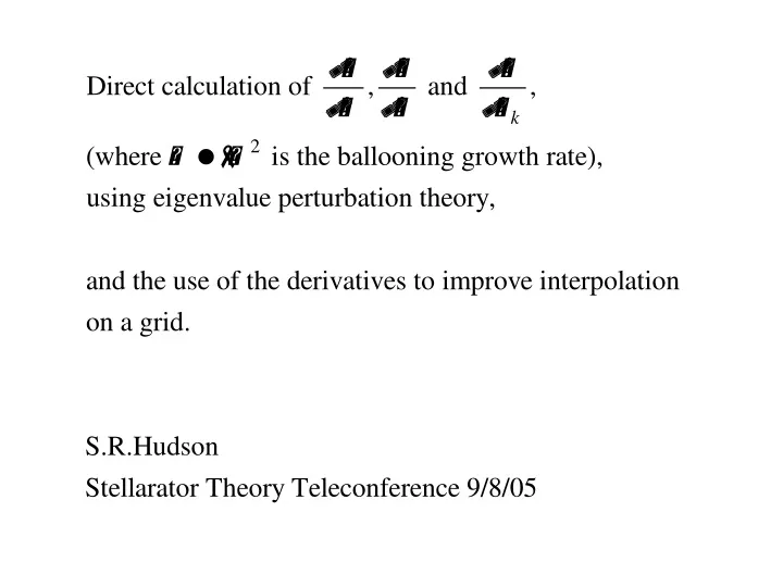
Alternatively, the eigenvalue derivatives can be determined directly using perturbation theory
The direct calculation of the derivatives is beneficial because . . . • The rays may be integrated directly • the data-cube need not be constructed • the eigenvalue derivatives may be given directly to an o.d.e. integrator • this may be useful if only a few ray trajectories are required • simple to locally refine ray trajectories using higher numerical accuracy • The calculation of the derivatives is consistent with the calculation of the eigenvalue (I need to work on this : eigenvalue and derivative are both extrapolated; are they still consistent ?) • The derivatives enable a higher order interpolation of the data-cube. • Consider a 2 point interpolation in 1 dimension,
For example, consider a tokamak • A circular cross section tokamak is simple • there is no dependence, minimal #Fourier harmonics • note that the ballooning code, interpolation, ray tracing etc. is fully 3D • Shown below are unstable ballooning contours
In 3D, 4th order interpolation is easily obtained eigenvalue interpolation error derivative interpolation error
The use of the derivatives enables a crude-grid to give good interpolation solid : exact calculated at 100 radial points dashed : 2-point interpolation ballooning profile X : grid points X : grid points radial (VMEC) coordinate
Future work possibly includes . . . • the eigenvalue and derivatives are calculated using Richardson’s extrapolation; • extrapolation wrt #grid points along field line for each ballooning calculation • need to check the consistency of extrapolated-eigenvalue with extrapolated-derivatives • higher order interpolation on data-cube grid • eg: extend 23 point interpolation to 43 interpolation: O(h4)O(h?) • higher order derivatives can be calculated using perturbation theory • higher order derivatives can further improve the data-cube interpolation • is it worthwhile to calculate the higher order derivatives ? • study some configurations of interest • need to understand the theory in more detail !!! • probably start with axisymmetric approximation, slowly add non-axisymmetry towards NCSX • appropriate mass normalization for comparison with CAS3D / TERPSICHORE • include FLR effects